bezier.hazmat.clipping module
Proof-of-concept for Bézier clipping.
The Bézier clipping algorithm is used to intersect two planar Bézier curves. It proceeds by using “fat lines” to recursively prune the region of accepted parameter ranges until the ranges converge to points. (A “fat line” is a rectangular region of a bounded distance from the line connecting the start and end points of a Bézier curve.)
It has quadratic convergence. It can be used to find tangent intersections,
which is the primary usage within bezier.
- bezier.hazmat.clipping.compute_implicit_line(nodes)
Compute the implicit form of the line connecting curve endpoints.
Note
This assumes, but does not check, that the first and last node in
nodesare different.Computes \(a, b\) and \(c\) in the implicit equation for the line
\[ax + by + c = 0\]In cases where the line is normalized (\(a^2 + b^2 = 1\), only unique up to sign), the function \(d(x, y) = ax + by + c\) can be used to determine the point-line distance from a point \(\left[\begin{array}{c} x \\ y \end{array}\right]\) to the line.
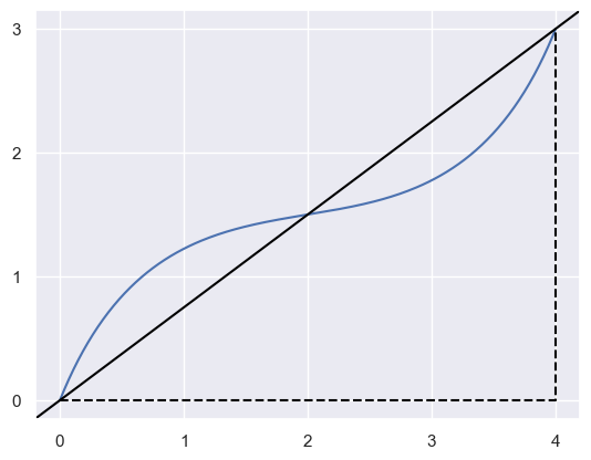
>>> import numpy as np
>>> nodes = np.asfortranarray([
...     [0.0, 1.0, 3.0, 4.0],
...     [0.0, 2.5, 0.5, 3.0],
... ])
>>> coeff_a, coeff_b, coeff_c = compute_implicit_line(nodes)
>>> float(coeff_a), float(coeff_b), float(coeff_c)
(-3.0, 4.0, 0.0)
- Parameters:
nodes (numpy.ndarray) –
2 x Narray of nodes in a curve. The line will be (directed) from the first to last node innodes.- Returns:
The triple of
The \(x\) coefficient \(a\)
The \(y\) coefficient \(b\)
The constant \(c\)
- Return type:
- bezier.hazmat.clipping.compute_fat_line(nodes)
Compute the “fat line” around a Bézier curve.
Both computes the implicit form
\[ax + by + c = 0\]for the line connecting the first and last node in
nodes. Also computes the maximum and minimum (non-normalized) distances to that line from each control point where (non-normalized) distance \(d\) is computed as \(d_i = a x_i + b y_i + c\). (To make \(d\) a true measure of Euclidean distance the line would need to be normalized so that \(a^2 + b^2 = 1\).)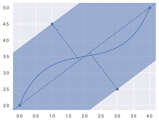
>>> nodes = np.asfortranarray([
...     [0.0, 1.0, 3.0, 4.0],
...     [2.0, 4.5, 2.5, 5.0],
... ])
>>> coeff_a, coeff_b, coeff_c, d_min, d_max = compute_fat_line(nodes)
>>> float(coeff_a), float(coeff_b), float(coeff_c)
(-3.0, 4.0, -8.0)
>>> float(d_min), float(d_max)
(-7.0, 7.0)
- Parameters:
nodes (numpy.ndarray) –
2 x Narray of nodes in a curve.- Returns:
The 5-tuple of
The \(x\) coefficient \(a\)
The \(y\) coefficient \(b\)
The constant \(c\)
The “minimum” (non-normalized) distance to the fat line among the control points.
The “maximum” (non-normalized) distance to the fat line among the control points.
- Return type:
- bezier.hazmat.clipping.clip_range(nodes1, nodes2)
Reduce the parameter range where two curves can intersect.
Note
This assumes, but does not check that the curves being considered will only have one intersection in the parameter ranges \(s \in \left[0, 1\right]\), \(t \in \left[0, 1\right]\). This assumption is based on the fact that Bézier clipping is meant to be used (within this library) to find tangent intersections for already subdivided (i.e. sufficiently zoomed in) curve segments.
Two Bézier curves \(B_1(s)\) and \(B_2(t)\) are defined by
nodes1andnodes2. The “fat line” (seecompute_fat_line()) for \(B_1(s)\) is used to narrow the range of possible \(t\)-values in an intersection by considering the (non-normalized) distance polynomial for \(B_2(t)\):\[d(t) = \sum_{j = 0}^m \binom{m}{j} t^j (1 - t)^{m - j} \cdot d_j\]Here \(d_j = a x_j + b y_j + c\) are the (non-normalized) distances of each control point \(\left[\begin{array}{c} x_j \\ y_j \end{array}\right]\) of \(B_2(t)\) to the implicit line for \(B_1(s)\).
Consider the following pair of Bézier curves and the distances from all of the control points to the implicit line for \(B_1(s)\):
>>> nodes1
array([[2. , 4.5, 2.5, 5. ],
       [0. , 1. , 3. , 4. ]])
>>> nodes2
array([[-0.25 ,  3.75 ,  7.   ],
       [ 3.125,  0.875,  3.125]])
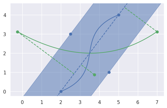
The (non-normalized) distances from the control points of \(B_2(t)\) define the distance polynomial \(d(t)\). By writing this polynomial as a Bézier curve, a convex hull can be formed. The intersection of this convex hull with the “fat line” of \(B_1(s)\) determines the extreme \(t\) values possible and allows clipping the range of \(B_2(t)\):
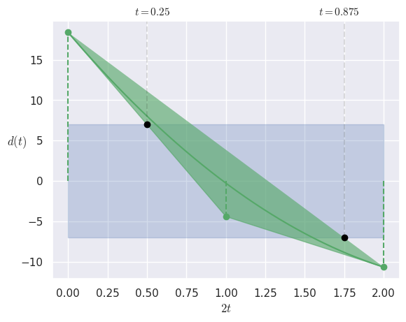
>>> s_min, s_max = clip_range(nodes1, nodes2)
>>> float(s_min), float(s_max)
(0.25, 0.875)
- Parameters:
nodes1 (numpy.ndarray) –
2 x N1array of nodes in a curve which will define the clipping region.nodes2 (numpy.ndarray) –
2 x N2array of nodes in a curve which will be clipped.
- Returns:
The pair of
The start parameter of the clipped range.
The end parameter of the clipped range.
- Return type: