bezier.curved_polygon module

Curved polygon and associated helpers.

A curved polygon (in \(\mathbf{R}^2\)) is defined by the collection of Bézier curves that determine the boundary.

class bezier.curved_polygon.CurvedPolygon(*edges, **kwargs)

Bases: object

Represents an object defined by its curved boundary.

The boundary is a piecewise defined collection of Bézier curves.

Note

The direction of the nodes in each Curve on the boundary is important. When verifying, we check that one curve begins where the last one ended.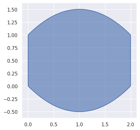

>>> import bezier
>>> import numpy as np
>>> nodes0 = np.asfortranarray([
...     [0.0,  1.0, 2.0],
...     [0.0, -1.0, 0.0],
... ])
>>> edge0 = bezier.Curve(nodes0, degree=2)
>>> nodes1 = np.asfortranarray([
...     [2.0, 2.0],
...     [0.0, 1.0],
... ])
>>> edge1 = bezier.Curve(nodes1, degree=1)
>>> nodes2 = np.asfortranarray([
...     [2.0, 1.0, 0.0],
...     [1.0, 2.0, 1.0],
... ])
>>> edge2 = bezier.Curve(nodes2, degree=2)
>>> nodes3 = np.asfortranarray([
...     [0.0, 0.0],
...     [1.0, 0.0],
... ])
>>> edge3 = bezier.Curve(nodes3, degree=1)
>>> curved_poly = bezier.CurvedPolygon(
...     edge0, edge1, edge2, edge3)
>>> curved_poly
<CurvedPolygon (num_sides=4)>

Though the endpoints of each pair of edges are verified to match, the curved polygon as a whole is not verified, so creating a curved polygon with self-intersections is possible:

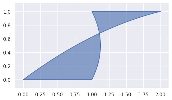
>>> nodes0 = np.asfortranarray([
...     [0.0, 1.0],
...     [0.0, 0.0],
... ])
>>> edge0 = bezier.Curve(nodes0, degree=1)
>>> nodes1 = np.asfortranarray([
...     [1.0, 1.25, 1.0],
...     [0.0, 0.5 , 1.0],
... ])
>>> edge1 = bezier.Curve(nodes1, degree=2)
>>> nodes2 = np.asfortranarray([
...     [1.0, 2.0],
...     [1.0, 1.0],
... ])
>>> edge2 = bezier.Curve(nodes2, degree=1)
>>> nodes3 = np.asfortranarray([
...     [2.0, 1.0 , 0.0],
...     [1.0, 0.75, 0.0]
... ])
>>> edge3 = bezier.Curve(nodes3, degree=2)
>>> curved_poly = bezier.CurvedPolygon(
...     edge0, edge1, edge2, edge3)
>>> curved_poly
<CurvedPolygon (num_sides=4)>

Parameters:

• edges (TupleCurve, …) – The boundary edges of the curved polygon.
• kwargs –

  There are two keyword arguments accepted:

  • metadata (Sequence): A sequence of triples associated with this curved polygon. This is intended to be used by callers that have created a curved polygon as an intersection between two Bézier triangles.
  • verify (bool): Indicates if the edges should be verified as having shared endpoints. Defaults to True.

  Other keyword arguments specified will be silently ignored.

property num_sides

The number of sides in the current polygon.

Type:int

property area

The area of the current curved polygon.

This assumes, but does not check, that the current curved polygon is valid (i.e. it is bounded by the edges).

This computes the area via Green’s theorem. Using the vector field \(\mathbf{F} = \left[-y, x\right]^T\), since \(\partial_x(x) - \partial_y(-y) = 2\) Green’s theorem says

\[\int_{\mathcal{P}} 2 \, d\textbf{x} = \int_{\partial \mathcal{P}} -y \, dx + x \, dy\]

(where \(\mathcal{P}\) is the current curved polygon).

Note that for a given edge \(C(r)\) with control points \(x_j, y_j\), the integral can be simplified:

\[\int_C -y \, dx + x \, dy = \int_0^1 (x y' - y x') \, dr = \sum_{i < j} (x_i y_j - y_i x_j) \int_0^1 b_{i, d} b'_{j, d} \, dr\]

where \(b_{i, d}, b_{j, d}\) are Bernstein basis polynomials.

Returns:The area of the current curved polygon. Return type:float

plot(pts_per_edge, color=None, ax=None, alpha=0.625)

Plot the current curved polygon.

Parameters:

• pts_per_edge (int) – Number of points to plot per curved edge.
• color (OptionalTuplefloat, float, float) – Color as RGB profile.
• ax (Optionalmatplotlib.artist.Artist) – matplotlib axis object to add plot to.
• alpha (Optionalfloat) – Alpha value of patch center, between 0 and 1 inclusive.

Returns:

The axis containing the plot. This may be a newly created axis.

Return type:

matplotlib.artist.Artist