bezier.curve module

Helper for Bézier Curves.

See Curve-Curve Intersection for examples using the Curve class to find intersections.

class bezier.curve.Curve(nodes, degree, *, copy=True, verify=True)

Bases: Base

Represents a Bézier curve.

We take the traditional definition: a Bézier curve is a mapping from \(s \in \left[0, 1\right]\) to convex combinations of points \(v_0, v_1, \ldots, v_n\) in some vector space:

\[B(s) = \sum_{j = 0}^n \binom{n}{j} s^j (1 - s)^{n - j} \cdot v_j\]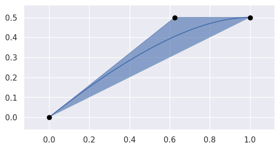

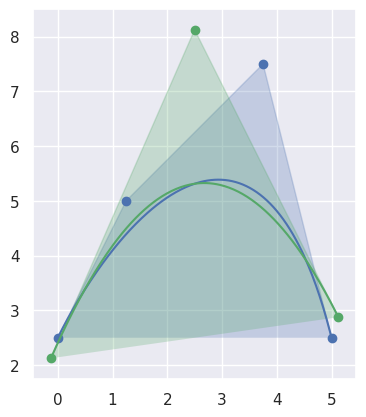
>>> import bezier
>>> import numpy as np
>>> nodes = np.asfortranarray([
...     [0.0, 0.625, 1.0],
...     [0.0, 0.5  , 0.5],
... ])
>>> curve = bezier.Curve(nodes, degree=2)
>>> curve
<Curve (degree=2, dimension=2)>

Parameters:

nodes (SequenceSequencenumbers.Number) – The nodes in the curve. Must be convertible to a 2D NumPy array of floating point values, where the columns represent each node while the rows are the dimension of the ambient space.
degree (int) – The degree of the curve. This is assumed to correctly correspond to the number of nodes. Use from_nodes() if the degree has not yet been computed.
copy (bool) – Flag indicating if the nodes should be copied before being stored. Defaults to True since callers may freely mutate nodes after passing in.
verify (bool) – Flag indicating if the degree should be verified against the number of nodes. Defaults to True.

classmethod from_nodes(nodes, copy=True)

Create a Curve from nodes.

Computes the degree based on the shape of nodes.

Parameters:	nodes (`SequenceSequencenumbers.Number`) – The nodes in the curve. Must be convertible to a 2D NumPy array of floating point values, where the columns represent each node while the rows are the dimension of the ambient space. copy (bool) – Flag indicating if the nodes should be copied before being stored. Defaults to `True` since callers may freely mutate `nodes` after passing in.
Returns:	The constructed curve.
Return type:	Curve

property length

The length of the current curve.

Computes the length via:

\[\int_{B\left(\left[0, 1\right]\right)} 1 \, d\mathbf{x} = \int_0^1 \left\lVert B'(s) \right\rVert_2 \, ds\]

Returns:	The length of the current curve.
Return type:	float

copy()

Make a copy of the current curve.

Returns:	Copy of current curve.
Return type:	Curve

evaluate(s)

Evaluate \(B(s)\) along the curve.

This method acts as a (partial) inverse to locate().

See evaluate_multi() for more details.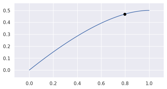

>>> nodes = np.asfortranarray([
...     [0.0, 0.625, 1.0],
...     [0.0, 0.5  , 0.5],
... ])
>>> curve = bezier.Curve(nodes, degree=2)
>>> curve.evaluate(0.75)
array([[0.796875],
       [0.46875 ]])

Parameters:	s (float) – Parameter along the curve.
Returns:	The point on the curve (as a two dimensional NumPy array with a single column).
Return type:	numpy.ndarray

evaluate_multi(s_vals)

Evaluate \(B(s)\) for multiple points along the curve.

This is done via a modified Horner’s method (vectorized for each s-value).

>>> nodes = np.asfortranarray([
...     [0.0, 1.0],
...     [0.0, 2.0],
...     [0.0, 3.0],
... ])
>>> curve = bezier.Curve(nodes, degree=1)
>>> curve
<Curve (degree=1, dimension=3)>
>>> s_vals = np.linspace(0.0, 1.0, 5)
>>> curve.evaluate_multi(s_vals)
array([[0.  , 0.25, 0.5 , 0.75, 1.  ],
       [0.  , 0.5 , 1.  , 1.5 , 2.  ],
       [0.  , 0.75, 1.5 , 2.25, 3.  ]])

Parameters:	s_vals (numpy.ndarray) – Parameters along the curve (as a 1D array).
Returns:	The points on the curve. As a two dimensional NumPy array, with the columns corresponding to each `s` value and the rows to the dimension.
Return type:	numpy.ndarray

evaluate_hodograph(s)

Evaluate the tangent vector \(B'(s)\) along the curve.

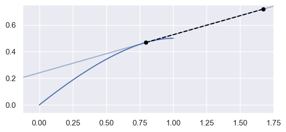
../../_images/curve_evaluate_hodograph.png

>>> nodes = np.asfortranarray([
...     [0.0, 0.625, 1.0],
...     [0.0, 0.5  , 0.5],
... ])
>>> curve = bezier.Curve(nodes, degree=2)
>>> curve.evaluate_hodograph(0.75)
array([[0.875],
       [0.25 ]])

Parameters:	s (float) – Parameter along the curve.
Returns:	The tangent vector along the curve (as a two dimensional NumPy array with a single column).
Return type:	numpy.ndarray

plot(num_pts, color=None, alpha=None, ax=None)

Plot the current curve.

Parameters:	num_pts (int) – Number of points to plot. color (`OptionalTuplefloat`, `float`, `float`) – Color as RGB profile. alpha (`Optionalfloat`) – The alpha channel for the color. ax (`Optionalmatplotlib.artist.Artist`) – matplotlib axis object to add plot to.
Returns:	The axis containing the plot. This may be a newly created axis.
Return type:	matplotlib.artist.Artist
Raises:	NotImplementedError – If the curve’s dimension is not `2`.

subdivide()

Split the curve \(B(s)\) into a left and right half.

Takes the interval \(\left[0, 1\right]\) and splits the curve into \(B_1 = B\left(\left[0, \frac{1}{2}\right]\right)\) and \(B_2 = B\left(\left[\frac{1}{2}, 1\right]\right)\). In order to do this, also reparameterizes the curve, hence the resulting left and right halves have new nodes.

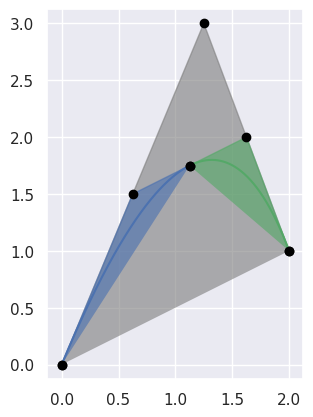
>>> nodes = np.asfortranarray([
...     [0.0, 1.25, 2.0],
...     [0.0, 3.0 , 1.0],
... ])
>>> curve = bezier.Curve(nodes, degree=2)
>>> left, right = curve.subdivide()
>>> left.nodes
array([[0.   , 0.625, 1.125],
       [0.   , 1.5  , 1.75 ]])
>>> right.nodes
array([[1.125, 1.625, 2.   ],
       [1.75 , 2.   , 1.   ]])

Returns:	The left and right sub-curves.
Return type:	`TupleCurve`, `Curve`

intersect(other, strategy=IntersectionStrategy.GEOMETRIC, verify=True)

Find the points of intersection with another curve.

See Curve-Curve Intersection for more details.

>>> nodes1 = np.asfortranarray([
...     [0.0, 0.375, 0.75 ],
...     [0.0, 0.75 , 0.375],
... ])
>>> curve1 = bezier.Curve(nodes1, degree=2)
>>> nodes2 = np.asfortranarray([
...     [0.5, 0.5 ],
...     [0.0, 0.75],
... ])
>>> curve2 = bezier.Curve(nodes2, degree=1)
>>> intersections = curve1.intersect(curve2)
>>> 3.0 * intersections
array([[2.],
       [2.]])
>>> s_vals = intersections[0, :]
>>> curve1.evaluate_multi(s_vals)
array([[0.5],
       [0.5]])

Parameters:	other (Curve) – Other curve to intersect with. strategy (`OptionalIntersectionStrategy`) – The intersection algorithm to use. Defaults to geometric. verify (`Optionalbool`) – Indicates if extra caution should be used to verify assumptions about the input and current curve. Can be disabled to speed up execution time. Defaults to `True`.
Returns:	`2 x N` array of `s`- and `t`-parameters where intersections occur (possibly empty).
Return type:	numpy.ndarray
Raises:	TypeError – If `other` is not a curve (and `verify=True`). NotImplementedError – If at least one of the curves isn’t two-dimensional (and `verify=True`). ValueError – If `strategy` is not a valid `IntersectionStrategy`.

self_intersections(strategy=IntersectionStrategy.GEOMETRIC, verify=True)

Find the points where the curve intersects itself.

For curves in general position, there will be no self-intersections:

>>> nodes = np.asfortranarray([
...     [0.0, 1.0, 0.0],
...     [0.0, 1.0, 2.0],
... ])
>>> curve = bezier.Curve(nodes, degree=2)
>>> curve.self_intersections()
array([], shape=(2, 0), dtype=float64)

However, some curves do have self-intersections. Consider a cubic with

\[B\left(\frac{3 - \sqrt{5}}{6}\right) = B\left(\frac{3 + \sqrt{5}}{6}\right)\]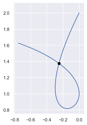

>>> nodes = np.asfortranarray([
...     [0.0, -1.0, 1.0, -0.75 ],
...     [2.0,  0.0, 1.0,  1.625],
... ])
>>> curve = bezier.Curve(nodes, degree=3)
>>> self_intersections = curve.self_intersections()
>>> sq5 = np.sqrt(5.0)
>>> expected = np.asfortranarray([
...     [3 - sq5],
...     [3 + sq5],
... ]) / 6.0
>>> max_err = np.max(np.abs(self_intersections - expected))
>>> binary_exponent(max_err)
-53

Some (somewhat pathological) curves can have multiple self-intersections, though the number possible is largely constrained by the degree. For example, this degree six curve has two self-intersections:

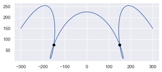
>>> nodes = np.asfortranarray([
...     [-300.0, 227.5 ,  -730.0,    0.0 ,   730.0, -227.5 , 300.0],
...     [ 150.0, 953.75, -2848.0, 4404.75, -2848.0,  953.75, 150.0],
... ])
>>> curve = bezier.Curve(nodes, degree=6)
>>> self_intersections = curve.self_intersections()
>>> 6.0 * self_intersections
array([[1., 4.],
       [2., 5.]])
>>> curve.evaluate_multi(self_intersections[:, 0])
array([[-150., -150.],
       [  75.,   75.]])
>>> curve.evaluate_multi(self_intersections[:, 1])
array([[150., 150.],
       [ 75.,  75.]])

Parameters:	strategy (`OptionalIntersectionStrategy`) – The intersection algorithm to use. Defaults to geometric. verify (`Optionalbool`) – Indicates if extra caution should be used to verify assumptions about the current curve. Can be disabled to speed up execution time. Defaults to `True`.
Returns:	`2 x N` array of `s1`- and `s2`-parameters where self-intersections occur (possibly empty). For each pair we have \(s_1 \neq s_2\) and \(B(s_1) = B(s_2)\).
Return type:	numpy.ndarray
Raises:	NotImplementedError – If the curve isn’t two-dimensional (and `verify=True`). NotImplementedError – If `strategy` is not `GEOMETRIC`.

elevate()

Return a degree-elevated version of the current curve.

Does this by converting the current nodes \(v_0, \ldots, v_n\) to new nodes \(w_0, \ldots, w_{n + 1}\) where

\[\begin{split}\begin{align*} w_0 &= v_0 \\ w_j &= \frac{j}{n + 1} v_{j - 1} + \frac{n + 1 - j}{n + 1} v_j \\ w_{n + 1} &= v_n \end{align*}\end{split}\]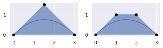

>>> nodes = np.asfortranarray([
...     [0.0, 1.5, 3.0],
...     [0.0, 1.5, 0.0],
... ])
>>> curve = bezier.Curve(nodes, degree=2)
>>> elevated = curve.elevate()
>>> elevated
<Curve (degree=3, dimension=2)>
>>> elevated.nodes
array([[0., 1., 2., 3.],
       [0., 1., 1., 0.]])

Returns:	The degree-elevated curve.
Return type:	Curve

reduce_()

Return a degree-reduced version of the current curve.

Does this by converting the current nodes \(v_0, \ldots, v_n\) to new nodes \(w_0, \ldots, w_{n - 1}\) that correspond to reversing the elevate() process.

This uses the pseudo-inverse of the elevation matrix. For example when elevating from degree 2 to 3, the matrix \(E_2\) is given by

\[\begin{split}\mathbf{v} = \left[\begin{array}{c c c} v_0 & v_1 & v_2 \end{array}\right] \longmapsto \left[\begin{array}{c c c c} v_0 & \frac{v_0 + 2 v_1}{3} & \frac{2 v_1 + v_2}{3} & v_2 \end{array}\right] = \frac{1}{3} \mathbf{v} \left[\begin{array}{c c c c} 3 & 1 & 0 & 0 \\ 0 & 2 & 2 & 0 \\ 0 & 0 & 1 & 3 \end{array}\right]\end{split}\]

and the (right) pseudo-inverse is given by

\[\begin{split}R_2 = E_2^T \left(E_2 E_2^T\right)^{-1} = \frac{1}{20} \left[\begin{array}{c c c} 19 & -5 & 1 \\ 3 & 15 & -3 \\ -3 & 15 & 3 \\ 1 & -5 & 19 \end{array}\right].\end{split}\]

Warning

Though degree-elevation preserves the start and end nodes, degree reduction has no such guarantee. Rather, the nodes produced are “best” in the least squares sense (when solving the normal equations).

>>> nodes = np.asfortranarray([
...     [-3.0, 0.0, 1.0, 0.0],
...     [ 3.0, 2.0, 3.0, 6.0],
... ])
>>> curve = bezier.Curve(nodes, degree=3)
>>> reduced = curve.reduce_()
>>> reduced
<Curve (degree=2, dimension=2)>
>>> reduced.nodes
array([[-3. ,  1.5,  0. ],
       [ 3. ,  1.5,  6. ]])

In the case that the current curve is not degree-elevated.

>>> nodes = np.asfortranarray([
...     [0.0, 1.25, 3.75, 5.0],
...     [2.5, 5.0 , 7.5 , 2.5],
... ])
>>> curve = bezier.Curve(nodes, degree=3)
>>> reduced = curve.reduce_()
>>> reduced
<Curve (degree=2, dimension=2)>
>>> reduced.nodes
array([[-0.125,  2.5  ,  5.125],
       [ 2.125,  8.125,  2.875]])

Returns:	The degree-reduced curve.
Return type:	Curve

specialize(start, end)

Specialize the curve to a given sub-interval.

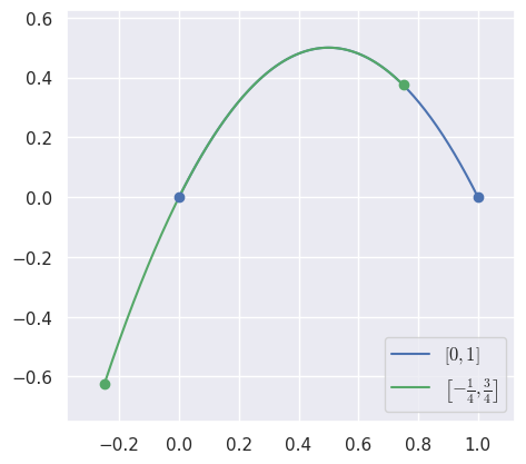
>>> nodes = np.asfortranarray([
...     [0.0, 0.5, 1.0],
...     [0.0, 1.0, 0.0],
... ])
>>> curve = bezier.Curve(nodes, degree=2)
>>> new_curve = curve.specialize(-0.25, 0.75)
>>> new_curve.nodes
array([[-0.25 ,  0.25 ,  0.75 ],
       [-0.625,  0.875,  0.375]])

This is a generalized version of subdivide(), and can even match the output of that method:

>>> left, right = curve.subdivide()
>>> also_left = curve.specialize(0.0, 0.5)
>>> np.all(also_left.nodes == left.nodes)
True
>>> also_right = curve.specialize(0.5, 1.0)
>>> np.all(also_right.nodes == right.nodes)
True

Parameters:	start (float) – The start point of the interval we are specializing to. end (float) – The end point of the interval we are specializing to.
Returns:	The newly-specialized curve.
Return type:	Curve

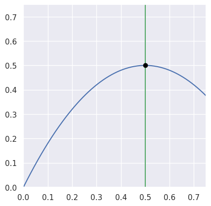
locate(point)

Find a point on the current curve.

Solves for \(s\) in \(B(s) = p\).

This method acts as a (partial) inverse to evaluate().

Note

A unique solution is only guaranteed if the current curve has no self-intersections. This code assumes, but doesn’t check, that this is true.

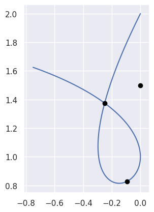
>>> nodes = np.asfortranarray([
...     [0.0, -1.0, 1.0, -0.75 ],
...     [2.0,  0.0, 1.0,  1.625],
... ])
>>> curve = bezier.Curve(nodes, degree=3)
>>> point1 = np.asfortranarray([
...     [-0.09375 ],
...     [ 0.828125],
... ])
>>> curve.locate(point1)
0.5
>>> point2 = np.asfortranarray([
...     [0.0],
...     [1.5],
... ])
>>> curve.locate(point2) is None
True
>>> point3 = np.asfortranarray([
...     [-0.25 ],
...     [ 1.375],
... ])
>>> curve.locate(point3) is None
Traceback (most recent call last):
  ...
ValueError: Parameters not close enough to one another

Parameters:	point (numpy.ndarray) – A (`D x 1`) point on the curve, where \(D\) is the dimension of the curve.
Returns:	The parameter value (\(s\)) corresponding to `point` or `None` if the point is not on the `curve`.
Return type:	`Optionalfloat`
Raises:	ValueError – If the dimension of the `point` doesn’t match the dimension of the current curve.

to_symbolic()

Convert to a SymPy matrix representing \(B(s)\).

Note

This method requires SymPy.

>>> nodes = np.asfortranarray([
...     [0.0, -1.0, 1.0, -0.75 ],
...     [2.0,  0.0, 1.0,  1.625],
... ])
>>> curve = bezier.Curve(nodes, degree=3)
>>> curve.to_symbolic()
Matrix([
[               -3*s*(3*s - 2)**2/4],
[-(27*s**3 - 72*s**2 + 48*s - 16)/8]])

Returns:	The curve \(B(s)\).
Return type:	`sympy.Matrix`

implicitize()

Implicitize the curve.

Note

This method requires SymPy.

>>> nodes = np.asfortranarray([
...     [0.0, 1.0, 1.0],
...     [2.0, 0.0, 1.0],
... ])
>>> curve = bezier.Curve(nodes, degree=2)
>>> curve.implicitize()
9*x**2 + 6*x*y - 20*x + y**2 - 8*y + 12

Returns:	The function that defines the curve in \(\mathbf{R}^2\) via \(f(x, y) = 0\).
Return type:	`sympy.Expr`
Raises:	ValueError – If the curve’s dimension is not `2`.

property degree

The degree of the current shape.

Type:	int

property dimension

The dimension that the shape lives in.

For example, if the shape lives in \(\mathbf{R}^3\), then the dimension is 3.

Type:	int

property nodes

The nodes that define the current shape.

Type:	numpy.ndarray