bezier.hazmat.intersection_helpers module
Pure Python helper methods for intersecting Bézier shapes.
- bezier.hazmat.intersection_helpers.ZERO_THRESHOLD = 0.0009765625
The bound below values are considered to be “too close” to
0.- Type:
- bezier.hazmat.intersection_helpers.MAX_NEWTON_ITERATIONS = 10
The maximum number of iterations for Newton’s method to converge.
- Type:
- bezier.hazmat.intersection_helpers.NEWTON_ERROR_RATIO = 1.4551915228366852e-11
Cap on error ratio during Newton’s method
Equal to \(2^{-36}\). See
newton_iterate()for more details.- Type:
- bezier.hazmat.intersection_helpers.newton_refine(s, nodes1, t, nodes2)
Apply one step of 2D Newton’s method.
Note
There is also a Fortran implementation of this function, which will be used if it can be built.
We want to use Newton’s method on the function
\[F(s, t) = B_1(s) - B_2(t)\]to refine \(\left(s_{\ast}, t_{\ast}\right)\). Using this, and the Jacobian \(DF\), we “solve”
\[\begin{split}\left[\begin{array}{c} 0 \\ 0 \end{array}\right] \approx F\left(s_{\ast} + \Delta s, t_{\ast} + \Delta t\right) \approx F\left(s_{\ast}, t_{\ast}\right) + \left[\begin{array}{c c} B_1'\left(s_{\ast}\right) & - B_2'\left(t_{\ast}\right) \end{array}\right] \left[\begin{array}{c} \Delta s \\ \Delta t \end{array}\right]\end{split}\]and refine with the component updates \(\Delta s\) and \(\Delta t\).
Note
This implementation assumes the curves live in \(\mathbf{R}^2\).
For example, the curves
\[\begin{split}\begin{align*} B_1(s) &= \left[\begin{array}{c} 0 \\ 0 \end{array}\right] (1 - s)^2 + \left[\begin{array}{c} 2 \\ 4 \end{array}\right] 2s(1 - s) + \left[\begin{array}{c} 4 \\ 0 \end{array}\right] s^2 \\ B_2(t) &= \left[\begin{array}{c} 2 \\ 0 \end{array}\right] (1 - t) + \left[\begin{array}{c} 0 \\ 3 \end{array}\right] t \end{align*}\end{split}\]intersect at the point \(B_1\left(\frac{1}{4}\right) = B_2\left(\frac{1}{2}\right) = \frac{1}{2} \left[\begin{array}{c} 2 \\ 3 \end{array}\right]\).
However, starting from the wrong point we have
\[\begin{split}\begin{align*} F\left(\frac{3}{8}, \frac{1}{4}\right) &= \frac{1}{8} \left[\begin{array}{c} 0 \\ 9 \end{array}\right] \\ DF\left(\frac{3}{8}, \frac{1}{4}\right) &= \left[\begin{array}{c c} 4 & 2 \\ 2 & -3 \end{array}\right] \\ \Longrightarrow \left[\begin{array}{c} \Delta s \\ \Delta t \end{array}\right] &= \frac{9}{64} \left[\begin{array}{c} -1 \\ 2 \end{array}\right]. \end{align*}\end{split}\]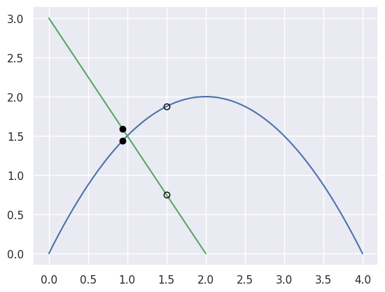
>>> import bezier
>>> import numpy as np
>>> nodes1 = np.asfortranarray([
...     [0.0, 2.0, 4.0],
...     [0.0, 4.0, 0.0],
... ])
>>> nodes2 = np.asfortranarray([
...     [2.0, 0.0],
...     [0.0, 3.0],
... ])
>>> s, t = 0.375, 0.25
>>> new_s, new_t = newton_refine(s, nodes1, t, nodes2)
>>> float(64.0 * (new_s - s))
-9.0
>>> float(64.0 * (new_t - t))
18.0
For “typical” curves, we converge to a solution quadratically. This means that the number of correct digits doubles every iteration (until machine precision is reached).
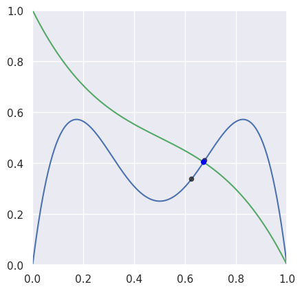
>>> nodes1 = np.asfortranarray([
...     [0.0, 0.25,  0.5, 0.75, 1.0],
...     [0.0, 2.0 , -2.0, 2.0 , 0.0],
... ])
>>> nodes2 = np.asfortranarray([
...     [0.0, 0.25, 0.5, 0.75, 1.0],
...     [1.0, 0.5 , 0.5, 0.5 , 0.0],
... ])
>>> # The expected intersection is the only real root of
>>> # 28 s^3 - 30 s^2 + 9 s - 1.
>>> expected, = realroots(28, -30, 9, -1)
>>> s_vals = [0.625, None, None, None, None]
>>> t = 0.625
>>> float(np.log2(abs(expected - s_vals[0])))
-4.399...
>>> s_vals[1], t = newton_refine(s_vals[0], nodes1, t, nodes2)
>>> float(np.log2(abs(expected - s_vals[1])))
-7.901...
>>> s_vals[2], t = newton_refine(s_vals[1], nodes1, t, nodes2)
>>> float(np.log2(abs(expected - s_vals[2])))
-16.010...
>>> s_vals[3], t = newton_refine(s_vals[2], nodes1, t, nodes2)
>>> float(np.log2(abs(expected - s_vals[3])))
-32.110...
>>> s_vals[4], t = newton_refine(s_vals[3], nodes1, t, nodes2)
>>> np.allclose(s_vals[4], expected, rtol=6 * machine_eps, atol=0.0)
True
However, when the intersection occurs at a point of tangency, the convergence becomes linear. This means that the number of correct digits added each iteration is roughly constant.
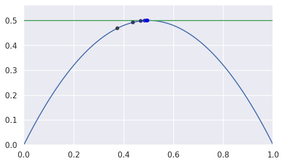
>>> nodes1 = np.asfortranarray([
...     [0.0, 0.5, 1.0],
...     [0.0, 1.0, 0.0],
... ])
>>> nodes2 = np.asfortranarray([
...     [0.0, 1.0],
...     [0.5, 0.5],
... ])
>>> expected = 0.5
>>> s_vals = [0.375, None, None, None, None, None]
>>> t = 0.375
>>> float(np.log2(abs(expected - s_vals[0])))
-3.0
>>> s_vals[1], t = newton_refine(s_vals[0], nodes1, t, nodes2)
>>> float(np.log2(abs(expected - s_vals[1])))
-4.0
>>> s_vals[2], t = newton_refine(s_vals[1], nodes1, t, nodes2)
>>> float(np.log2(abs(expected - s_vals[2])))
-5.0
>>> s_vals[3], t = newton_refine(s_vals[2], nodes1, t, nodes2)
>>> float(np.log2(abs(expected - s_vals[3])))
-6.0
>>> s_vals[4], t = newton_refine(s_vals[3], nodes1, t, nodes2)
>>> float(np.log2(abs(expected - s_vals[4])))
-7.0
>>> s_vals[5], t = newton_refine(s_vals[4], nodes1, t, nodes2)
>>> float(np.log2(abs(expected - s_vals[5])))
-8.0
Unfortunately, the process terminates with an error that is not close to machine precision \(\varepsilon\) when \(\Delta s = \Delta t = 0\).
>>> s1 = t1 = 0.5 - 0.5**27
>>> float(np.log2(0.5 - s1))
-27.0
>>> s2, t2 = newton_refine(s1, nodes1, t1, nodes2)
>>> bool(s2 == t2)
True
>>> float(np.log2(0.5 - s2))
-28.0
>>> s3, t3 = newton_refine(s2, nodes1, t2, nodes2)
>>> bool(s3 == t3 == s2)
True
Due to round-off near the point of tangency, the final error resembles \(\sqrt{\varepsilon}\) rather than machine precision as expected.
Note
The following is not implemented in this function. It’s just an exploration on how the shortcomings might be addressed.
However, this can be overcome. At the point of tangency, we want \(B_1'(s) \parallel B_2'(t)\). This can be checked numerically via
\[B_1'(s) \times B_2'(t) = 0.\]For the last example (the one that converges linearly), this is
\[\begin{split}0 = \left[\begin{array}{c} 1 \\ 2 - 4s \end{array}\right] \times \left[\begin{array}{c} 1 \\ 0 \end{array}\right] = 4 s - 2.\end{split}\]With this, we can modify Newton’s method to find a zero of the over-determined system
\[\begin{split}G(s, t) = \left[\begin{array}{c} B_0(s) - B_1(t) \\ B_1'(s) \times B_2'(t) \end{array}\right] = \left[\begin{array}{c} s - t \\ 2 s (1 - s) - \frac{1}{2} \\ 4 s - 2\end{array}\right].\end{split}\]Since \(DG\) is \(3 \times 2\), we can’t invert it. However, we can find a least-squares solution:
\[\begin{split}\left(DG^T DG\right) \left[\begin{array}{c} \Delta s \\ \Delta t \end{array}\right] = -DG^T G.\end{split}\]This only works if \(DG\) has full rank. In this case, it does since the submatrix containing the first and last rows has rank two:
\[\begin{split}DG = \left[\begin{array}{c c} 1 & -1 \\ 2 - 4 s & 0 \\ 4 & 0 \end{array}\right].\end{split}\]Though this avoids a singular system, the normal equations have a condition number that is the square of the condition number of the matrix.
Starting from \(s = t = \frac{3}{8}\) as above:
>>> s0, t0 = 0.375, 0.375
>>> float(np.log2(0.5 - s0))
-3.0
>>> s1, t1 = modified_update(s0, t0)
>>> s1 == t1
True
>>> 1040.0 * s1
519.0
>>> float(np.log2(0.5 - s1))
-10.022...
>>> s2, t2 = modified_update(s1, t1)
>>> s2 == t2
True
>>> float(np.log2(0.5 - s2))
-31.067...
>>> s3, t3 = modified_update(s2, t2)
>>> s3 == t3 == 0.5
True
- Parameters:
s (float) – Parameter of a near-intersection along the first curve.
nodes1 (numpy.ndarray) – Nodes of first curve forming intersection.
t (float) – Parameter of a near-intersection along the second curve.
nodes2 (numpy.ndarray) – Nodes of second curve forming intersection.
- Returns:
The refined parameters from a single Newton step.
- Return type:
- Raises:
ValueError – If the Jacobian is singular at
(s, t).
- class bezier.hazmat.intersection_helpers.NewtonSimpleRoot(nodes1, first_deriv1, nodes2, first_deriv2)
Bases:
objectCallable object that facilitates Newton’s method.
This is meant to be used to compute the Newton update via:
\[\begin{split}DF(s, t) \left[\begin{array}{c} \Delta s \\ \Delta t \end{array}\right] = -F(s, t).\end{split}\]- Parameters:
nodes1 (numpy.ndarray) – Control points of the first curve.
first_deriv1 (numpy.ndarray) – Control points of the curve \(B_1'(s)\).
nodes2 (numpy.ndarray) – Control points of the second curve.
first_deriv2 (numpy.ndarray) – Control points of the curve \(B_2'(t)\).
- class bezier.hazmat.intersection_helpers.NewtonDoubleRoot(nodes1, first_deriv1, second_deriv1, nodes2, first_deriv2, second_deriv2)
Bases:
objectCallable object that facilitates Newton’s method for double roots.
This is an augmented version of
NewtonSimpleRoot.For non-simple intersections (i.e. multiplicity greater than 1), the curves will be tangent, which forces \(B_1'(s) \times B_2'(t)\) to be zero. Unfortunately, that quantity is also equal to the determinant of the Jacobian, so \(DF\) will not be full rank.
In order to produce a system that can be solved, an an augmented function is computed:
\[\begin{split}G(s, t) = \left[\begin{array}{c} F(s, t) \\ \hline B_1'(s) \times B_2'(t) \end{array}\right]\end{split}\]The use of \(B_1'(s) \times B_2'(t)\) (with lowered degree in \(s\) and \(t\)) means that the rank deficiency in \(DF\) can be fixed in:
\[\begin{split}DG(s, t) = \left[\begin{array}{c | c} B_1'(s) & -B_2'(t) \\ \hline B_1''(s) \times B_2'(t) & B_1'(s) \times B_2''(t) \end{array}\right]\end{split}\](This may not always be full rank, but in the double root / multiplicity 2 case it will be full rank near a solution.)
Rather than finding a least squares solution to the overdetermined system
\[\begin{split}DG(s, t) \left[\begin{array}{c} \Delta s \\ \Delta t \end{array}\right] = -G(s, t)\end{split}\]we find a solution to the square (and hopefully full rank) system:
\[\begin{split}DG^T DG \left[\begin{array}{c} \Delta s \\ \Delta t \end{array}\right] = -DG^T G.\end{split}\]Forming \(DG^T DG\) squares the condition number, so it would be “better” to use
lstsq()(which wraps the LAPACK routinedgelsd). However, usingsolve2x2()is much more straightforward and in practice this is just as accurate.- Parameters:
nodes1 (numpy.ndarray) – Control points of the first curve.
first_deriv1 (numpy.ndarray) – Control points of the curve \(B_1'(s)\).
second_deriv1 (numpy.ndarray) – Control points of the curve \(B_1''(s)\).
nodes2 (numpy.ndarray) – Control points of the second curve.
first_deriv2 (numpy.ndarray) – Control points of the curve \(B_2'(t)\).
second_deriv2 (numpy.ndarray) – Control points of the curve \(B_2''(t)\).
- bezier.hazmat.intersection_helpers.newton_iterate(evaluate_fn, s, t)
Perform a Newton iteration.
Warning
In this function, we assume that \(s\) and \(t\) are nonzero, this makes convergence easier to detect since “relative error” at
0.0is not a useful measure.There are several tolerance / threshold quantities used below:
\(10\) (
MAX_NEWTON_ITERATIONS) iterations will be done before “giving up”. This is based on the assumption that we are already starting near a root, so quadratic convergence should terminate quickly.\(\tau = \frac{1}{4}\) is used as the boundary between linear and superlinear convergence. So if the current error \(\|p_{n + 1} - p_n\|\) is not smaller than \(\tau\) times the previous error \(\|p_n - p_{n - 1}\|\), then convergence is considered to be linear at that point.
\(\frac{2}{3}\) of all iterations must be converging linearly for convergence to be stopped (and moved to the next regime). This will only be checked after 4 or more updates have occurred.
\(\tau = 2^{-36}\) (
NEWTON_ERROR_RATIO) is used to determine that an update is sufficiently small to stop iterating. So if the error \(\|p_{n + 1} - p_n\|\) smaller than \(\tau\) times size of the term being updated \(\|p_n\|\), then we exit with the “correct” answer.
It is assumed that
evaluate_fnwill use a Jacobian return value ofNoneto indicate that \(F(s, t)\) is exactly0.0. We assume that if the function evaluates to exactly0.0, then we are at a solution. It is possible however, that badly parameterized curves can evaluate to exactly0.0for inputs that are relatively far away from a solution (see issue #21).- Parameters:
evaluate_fn (
CallableTuplefloat,float,TupleOptionalnumpy.ndarray,numpy.ndarray) – A callable which takes \(s\) and \(t\) and produces the (optional) Jacobian matrix (2 x 2) and an evaluated function (2 x 1) value.s (float) – The (first) parameter where the iteration will start.
t (float) – The (second) parameter where the iteration will start.
- Returns:
The triple of
Flag indicating if the iteration converged.
The current \(s\) value when the iteration stopped.
The current \(t\) value when the iteration stopped.
- Return type:
- bezier.hazmat.intersection_helpers.full_newton_nonzero(s, nodes1, t, nodes2)
Perform a Newton iteration until convergence to a solution.
This is the “implementation” for
full_newton(). In this function, we assume that \(s\) and \(t\) are nonzero.- Parameters:
s (float) – The parameter along the first curve where the iteration will start.
nodes1 (numpy.ndarray) – Control points of the first curve.
t (float) – The parameter along the second curve where the iteration will start.
nodes2 (numpy.ndarray) – Control points of the second curve.
- Returns:
The pair of \(s\) and \(t\) values that Newton’s method converged to.
- Return type:
- Raises:
NotImplementedError – If Newton’s method doesn’t converge in either the multiplicity 1 or 2 cases.
- bezier.hazmat.intersection_helpers.full_newton(s, nodes1, t, nodes2)
Perform a Newton iteration until convergence to a solution.
This assumes \(s\) and \(t\) are sufficiently close to an intersection. It does not govern the maximum distance away that the solution can lie, though the subdivided intervals that contain \(s\) and \(t\) could be used.
To avoid round-off issues near
0.0, this reverses the direction of a curve and replaces the parameter value \(\nu\) with \(1 - \nu\) whenever \(\nu < \tau\) (here we use a threshold \(\tau\) equal to \(2^{-10}\), i.e.ZERO_THRESHOLD).- Parameters:
s (float) – The parameter along the first curve where the iteration will start.
nodes1 (numpy.ndarray) – Control points of the first curve.
t (float) – The parameter along the second curve where the iteration will start.
nodes2 (numpy.ndarray) – Control points of the second curve.
- Returns:
The pair of \(s\) and \(t\) values that Newton’s method converged to.
- Return type:
- class bezier.hazmat.intersection_helpers.IntersectionClassification(value, names=<not given>, *values, module=None, qualname=None, type=None, start=1, boundary=None)
Bases:
EnumEnum classifying the “interior” curve in an intersection.
Provided as the output values for
classify_intersection().- FIRST = 0
The first curve is on the interior.
- SECOND = 1
The second curve is on the interior.
- OPPOSED = 2
Tangent intersection with opposed interiors.
- TANGENT_FIRST = 3
Tangent intersection, first curve is on the interior.
- TANGENT_SECOND = 4
Tangent intersection, second curve is on the interior.
- IGNORED_CORNER = 5
Intersection at a corner, interiors don’t intersect.
- TANGENT_BOTH = 6
Tangent intersection, both curves are interior from some perspective.
- COINCIDENT = 7
Intersection is actually an endpoint of a coincident segment.
- COINCIDENT_UNUSED = 8
Unused because the edges are moving in opposite directions.
- class bezier.hazmat.intersection_helpers.Intersection(index_first, s, index_second, t, interior_curve=None)
Bases:
objectRepresentation of a curve-curve intersection.
- Parameters:
index_first (int) – The index of the first curve within a list of curves. Expected to be used to index within the three edges of a triangle.
s (float) – The parameter along the first curve where the intersection occurs.
index_second (int) – The index of the second curve within a list of curves. Expected to be used to index within the three edges of a triangle.
t (float) – The parameter along the second curve where the intersection occurs.
interior_curve (
OptionalIntersectionClassification) – The classification of the intersection.
- interior_curve
Which of the curves is on the interior.
See
classify_intersection()for more details.
- class bezier.hazmat.intersection_helpers.IntersectionStrategy(value, names=<not given>, *values, module=None, qualname=None, type=None, start=1, boundary=None)
Bases:
EnumEnum determining the type of intersection algorithm to use.
- GEOMETRIC = 0
Geometric approach to intersection (via subdivision).
- ALGEBRAIC = 1
Algebraic approach to intersection (via implicitization).