bezier.hazmat.curve_helpers module¶

Pure Python implementations of helper methods for Bézier curves.

bezier.hazmat.curve_helpers.make_subdivision_matrices(degree)¶

Make the matrix used to subdivide a curve.

Note

This is a helper for subdivide_nodes(). It does not have a Fortran speedup because it is only used by a function which has a Fortran speedup.

Parameters: degree (int) – The degree of the curve.
Returns: The matrices used to convert the nodes into left and right nodes, respectively.
Return type: Tuple [ numpy.ndarray, numpy.ndarray ]

bezier.hazmat.curve_helpers.subdivide_nodes(nodes)¶

Subdivide a curve into two sub-curves.

Does so by taking the unit interval (i.e. the domain of the curve) and splitting it into two sub-intervals by splitting down the middle.

Note

There is also a Fortran implementation of this function, which will be used if it can be built.

Parameters: nodes (numpy.ndarray) – The nodes defining a Bézier curve.
Returns: The nodes for the two sub-curves.
Return type: Tuple [ numpy.ndarray, numpy.ndarray ]

bezier.hazmat.curve_helpers.evaluate_multi(nodes, s_vals)¶

Computes multiple points along a curve.

Does so via a modified Horner’s method for each value in s_vals rather than using the de Casteljau algorithm.

Note

There is also a Fortran implementation of this function, which will be used if it can be built.

Parameters

nodes (numpy.ndarray) – The nodes defining a curve.
s_vals (numpy.ndarray) – Parameters along the curve (as a 1D array).

Returns

The evaluated points on the curve as a two dimensional NumPy array, with the columns corresponding to each s value and the rows to the dimension.

Return type

numpy.ndarray

bezier.hazmat.curve_helpers.evaluate_multi_barycentric(nodes, lambda1, lambda2)¶

Evaluates a Bézier type-function.

Of the form

\[B(\lambda_1, \lambda_2) = \sum_j \binom{n}{j} \lambda_1^{n - j} \lambda_2^j \cdot v_j\]

for some set of vectors \(v_j\) given by nodes.

Does so via a modified Horner’s method for each pair of values in lambda1 and lambda2, rather than using the de Casteljau algorithm.

Note

There is also a Fortran implementation of this function, which will be used if it can be built.

Parameters

nodes (numpy.ndarray) – The nodes defining a curve.
lambda1 (numpy.ndarray) – Parameters along the curve (as a 1D array).
lambda2 (numpy.ndarray) – Parameters along the curve (as a 1D array). Typically we have lambda1 + lambda2 == 1.

Returns

The evaluated points as a two dimensional NumPy array, with the columns corresponding to each pair of parameter values and the rows to the dimension.

Return type

numpy.ndarray

bezier.hazmat.curve_helpers.vec_size(nodes, s_val)¶

Compute \(\|B(s)\|_2\).

Note

This is a helper for compute_length() and does not have a Fortran speedup.

Intended to be used with functools.partial() to fill in the value of nodes and create a callable that only accepts s_val.

Parameters

nodes (numpy.ndarray) – The nodes defining a curve.
s_val (float) – Parameter to compute \(B(s)\).

Returns

The norm of \(B(s)\).

Return type

float

bezier.hazmat.curve_helpers.compute_length(nodes)¶

Approximately compute the length of a curve.

If degree is \(n\), then the Hodograph curve \(B'(s)\) is degree \(d = n - 1\). Using this curve, we approximate the integral:

\[\int_{B\left(\left[0, 1\right]\right)} 1 \, d\mathbf{x} = \int_0^1 \left\lVert B'(s) \right\rVert_2 \, ds\]

using QUADPACK (via SciPy).

Note

There is also a Fortran implementation of this function, which will be used if it can be built.

Parameters: nodes (numpy.ndarray) – The nodes defining a curve.
Returns: The length of the curve.
Return type: float
Raises: ValueError – If nodes has zero columns.

bezier.hazmat.curve_helpers.elevate_nodes(nodes)¶

Degree-elevate a Bézier curve.

Does this by converting the current nodes \(v_0, \ldots, v_n\) to new nodes \(w_0, \ldots, w_{n + 1}\) where

\[\begin{split}\begin{align*} w_0 &= v_0 \\ w_j &= \frac{j}{n + 1} v_{j - 1} + \frac{n + 1 - j}{n + 1} v_j \\ w_{n + 1} &= v_n \end{align*}\end{split}\]

Note

There is also a Fortran implementation of this function, which will be used if it can be built.

Parameters: nodes (numpy.ndarray) – The nodes defining a curve.
Returns: The nodes of the degree-elevated curve.
Return type: numpy.ndarray

bezier.hazmat.curve_helpers.de_casteljau_one_round(nodes, lambda1, lambda2)¶

Perform one round of de Casteljau’s algorithm.

Note

This is a helper for specialize_curve(). It does not have a Fortran speedup because it is only used by a function which has a Fortran speedup.

The weights are assumed to sum to one.

Parameters

nodes (numpy.ndarray) – Control points for a curve.
lambda1 (float) – First barycentric weight on interval.
lambda2 (float) – Second barycentric weight on interval.

Returns

The nodes for a “blended” curve one degree lower.

Return type

numpy.ndarray

bezier.hazmat.curve_helpers.specialize_curve(nodes, start, end)¶

Specialize a curve to a re-parameterization

Note

This assumes the curve is degree 1 or greater but doesn’t check.

Note

There is also a Fortran implementation of this function, which will be used if it can be built.

Parameters

nodes (numpy.ndarray) – Control points for a curve.
start (float) – The start point of the interval we are specializing to.
end (float) – The end point of the interval we are specializing to.

Returns

The control points for the specialized curve.

Return type

numpy.ndarray

bezier.hazmat.curve_helpers.evaluate_hodograph(s, nodes)¶

Evaluate the Hodograph curve at a point \(s\).

The Hodograph (first derivative) of a Bézier curve degree \(d = n - 1\) and is given by

\[B'(s) = n \sum_{j = 0}^{d} \binom{d}{j} s^j (1 - s)^{d - j} \cdot \Delta v_j\]

where each forward difference is given by \(\Delta v_j = v_{j + 1} - v_j\).

Note

There is also a Fortran implementation of this function, which will be used if it can be built.

Parameters

nodes (numpy.ndarray) – The nodes of a curve.
s (float) – A parameter along the curve at which the Hodograph is to be evaluated.

Returns

The point on the Hodograph curve (as a two dimensional NumPy array with a single row).

Return type

numpy.ndarray

bezier.hazmat.curve_helpers.get_curvature(nodes, tangent_vec, s)¶

Compute the signed curvature of a curve at \(s\).

Computed via

\[\frac{B'(s) \times B''(s)}{\left\lVert B'(s) \right\rVert_2^3}\]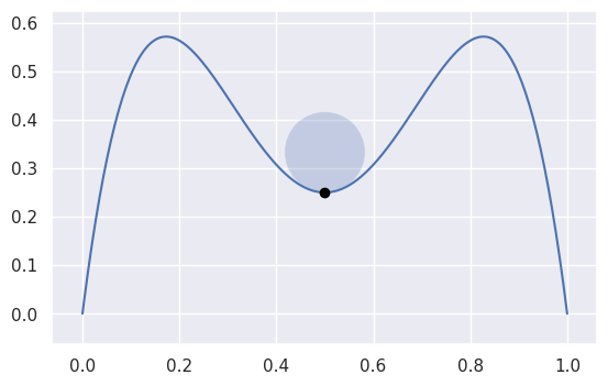

>>> nodes = np.asfortranarray([
...     [1.0, 0.75,  0.5, 0.25, 0.0],
...     [0.0, 2.0 , -2.0, 2.0 , 0.0],
... ])
>>> s = 0.5
>>> tangent_vec = evaluate_hodograph(s, nodes)
>>> tangent_vec
array([[-1.],
       [ 0.]])
>>> curvature = get_curvature(nodes, tangent_vec, s)
>>> curvature
-12.0

Note

There is also a Fortran implementation of this function, which will be used if it can be built.

Parameters

nodes (numpy.ndarray) – The nodes of a curve.
tangent_vec (numpy.ndarray) – The already computed value of \(B'(s)\)
s (float) – The parameter value along the curve.

Returns

The signed curvature.

Return type

float

bezier.hazmat.curve_helpers.newton_refine(nodes, point, s)¶

Refine a solution to \(B(s) = p\) using Newton’s method.

Computes updates via

\[\mathbf{0} \approx \left(B\left(s_{\ast}\right) - p\right) + B'\left(s_{\ast}\right) \Delta s\]

For example, consider the curve

\[\begin{split}B(s) = \left[\begin{array}{c} 0 \\ 0 \end{array}\right] (1 - s)^2 + \left[\begin{array}{c} 1 \\ 2 \end{array}\right] 2 (1 - s) s + \left[\begin{array}{c} 3 \\ 1 \end{array}\right] s^2\end{split}\]

and the point \(B\left(\frac{1}{4}\right) = \frac{1}{16} \left[\begin{array}{c} 9 \\ 13 \end{array}\right]\).

Starting from the wrong point \(s = \frac{3}{4}\), we have

\[\begin{split}\begin{align*} p - B\left(\frac{1}{2}\right) &= -\frac{1}{2} \left[\begin{array}{c} 3 \\ 1 \end{array}\right] \\ B'\left(\frac{1}{2}\right) &= \frac{1}{2} \left[\begin{array}{c} 7 \\ -1 \end{array}\right] \\ \Longrightarrow \frac{1}{4} \left[\begin{array}{c c} 7 & -1 \end{array}\right] \left[\begin{array}{c} 7 \\ -1 \end{array}\right] \Delta s &= -\frac{1}{4} \left[\begin{array}{c c} 7 & -1 \end{array}\right] \left[\begin{array}{c} 3 \\ 1 \end{array}\right] \\ \Longrightarrow \Delta s &= -\frac{2}{5} \end{align*}\end{split}\]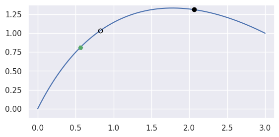

>>> nodes = np.asfortranarray([
...     [0.0, 1.0, 3.0],
...     [0.0, 2.0, 1.0],
... ])
>>> curve = bezier.Curve(nodes, degree=2)
>>> point = curve.evaluate(0.25)
>>> point
array([[0.5625],
       [0.8125]])
>>> s = 0.75
>>> new_s = newton_refine(nodes, point, s)
>>> 5 * (new_s - s)
-2.0

On curves that are not “valid” (i.e. \(B(s)\) is not injective with non-zero gradient), Newton’s method may break down and converge linearly:

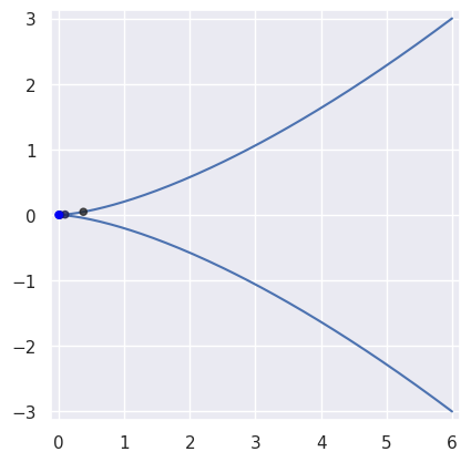
../../_images/newton_refine_curve_cusp.png

>>> nodes = np.asfortranarray([
...     [ 6.0, -2.0, -2.0, 6.0],
...     [-3.0,  3.0, -3.0, 3.0],
... ])
>>> curve = bezier.Curve(nodes, degree=3)
>>> expected = 0.5
>>> point = curve.evaluate(expected)
>>> point
array([[0.],
       [0.]])
>>> s_vals = [0.625, None, None, None, None, None]
>>> np.log2(abs(expected - s_vals[0]))
-3.0
>>> s_vals[1] = newton_refine(nodes, point, s_vals[0])
>>> np.log2(abs(expected - s_vals[1]))
-3.983...
>>> s_vals[2] = newton_refine(nodes, point, s_vals[1])
>>> np.log2(abs(expected - s_vals[2]))
-4.979...
>>> s_vals[3] = newton_refine(nodes, point, s_vals[2])
>>> np.log2(abs(expected - s_vals[3]))
-5.978...
>>> s_vals[4] = newton_refine(nodes, point, s_vals[3])
>>> np.log2(abs(expected - s_vals[4]))
-6.978...
>>> s_vals[5] = newton_refine(nodes, point, s_vals[4])
>>> np.log2(abs(expected - s_vals[5]))
-7.978...

Due to round-off, the Newton process terminates with an error that is not close to machine precision \(\varepsilon\) when \(\Delta s = 0\).

>>> s_vals = [0.625]
>>> new_s = newton_refine(nodes, point, s_vals[-1])
>>> while new_s not in s_vals:
...     s_vals.append(new_s)
...     new_s = newton_refine(nodes, point, s_vals[-1])
...
>>> terminal_s = s_vals[-1]
>>> terminal_s == newton_refine(nodes, point, terminal_s)
True
>>> 2.0**(-31) <= abs(terminal_s - 0.5) <= 2.0**(-28)
True

Due to round-off near the cusp, the final error resembles \(\sqrt{\varepsilon}\) rather than machine precision as expected.

Note

There is also a Fortran implementation of this function, which will be used if it can be built.

Parameters

nodes (numpy.ndarray) – The nodes defining a Bézier curve.
point (numpy.ndarray) – A point on the curve.
s (float) – An “almost” solution to \(B(s) = p\).

Returns

The updated value \(s + \Delta s\).

Return type

float

bezier.hazmat.curve_helpers.locate_point(nodes, point)¶

Locate a point on a curve.

Does so by recursively subdividing the curve and rejecting sub-curves with bounding boxes that don’t contain the point. After the sub-curves are sufficiently small, uses Newton’s method to zoom in on the parameter value.

Note

This assumes, but does not check, that point is D x 1, where D is the dimension that curve is in.

Note

There is also a Fortran implementation of this function, which will be used if it can be built.

Parameters

nodes (numpy.ndarray) – The nodes defining a Bézier curve.
point (numpy.ndarray) – The point to locate.

Returns

The parameter value (\(s\)) corresponding to point or None if the point is not on the curve.

Return type

Optional [ float ]

Raises

ValueError – If the standard deviation of the remaining start / end parameters among the subdivided intervals exceeds a given threshold (e.g. \(2^{-20}\)).

bezier.hazmat.curve_helpers.reduce_pseudo_inverse(nodes)¶

Performs degree-reduction for a Bézier curve.

Does so by using the pseudo-inverse of the degree elevation operator (which is overdetermined).

Note

There is also a Fortran implementation of this function, which will be used if it can be built.

Parameters: nodes (numpy.ndarray) – The nodes in the curve.
Returns: The reduced nodes.
Return type: numpy.ndarray
Raises: UnsupportedDegree – If the degree is not 1, 2, 3 or 4.

bezier.hazmat.curve_helpers.projection_error(nodes, projected)¶

Compute the error between nodes and the projected nodes.

Note

This is a helper for maybe_reduce(), which is in turn a helper for full_reduce(). Hence there is no corresponding Fortran speedup.

For now, just compute the relative error in the Frobenius norm. But, we may wish to consider the error per row / point instead.

Parameters

nodes (numpy.ndarray) – Nodes in a curve.
projected (numpy.ndarray) – The nodes projected into the space of degree-elevated nodes.

Returns

The relative error.

Return type

float

bezier.hazmat.curve_helpers.maybe_reduce(nodes)¶

Reduce nodes in a curve if they are degree-elevated.

Note

This is a helper for full_reduce(). Hence there is no corresponding Fortran speedup.

We check if the nodes are degree-elevated by projecting onto the space of degree-elevated curves of the same degree, then comparing to the projection. We form the projection by taking the corresponding (right) elevation matrix \(E\) (from one degree lower) and forming \(E^T \left(E E^T\right)^{-1} E\).

Parameters: nodes (numpy.ndarray) – The nodes in the curve.
Returns: Pair of values. The first indicates if the nodes were reduced. The second is the resulting nodes, either the reduced ones or the original passed in.
Return type: Tuple [ bool, numpy.ndarray ]
Raises: UnsupportedDegree – If the curve is degree 5 or higher.

bezier.hazmat.curve_helpers.full_reduce(nodes)¶

Apply degree reduction to nodes until it can no longer be reduced.

Note

There is also a Fortran implementation of this function, which will be used if it can be built.

Parameters: nodes (numpy.ndarray) – The nodes in the curve.
Returns: The fully degree-reduced nodes.
Return type: numpy.ndarray