curve module

This is a collection of procedures for performing computations on a Bézier curve.

Procedures

void BEZ_compute_length(const int *num_nodes, const int *dimension, const double *nodes, double *length, int *error_val)

Computes the length of a Bézier curve via

\[\ell = \int_0^1 \left\lVert B'(s) \right\rVert \, ds.\]

Parameters

• num_nodes (const int*) – [Input] The number of control points \(N\) of a Bézier curve.

• dimension (const int*) – [Input] The dimension \(D\) such that the curve lies in \(\mathbf{R}^D\).

• nodes (const double*) – [Input] The actual control points of the curve as a \(D \times N\) array. This should be laid out in Fortran order, with \(D N\) total values.

• length (double*) – [Output] The computed length \(\ell\).

• error_val (int*) – [Output] An error status passed along from dqagse (a QUADPACK procedure).

Signature:

void
BEZ_compute_length(const int *num_nodes,
                   const int *dimension,
                   const double *nodes,
                   double *length,
                   int *error_val);

Example:

// Inputs.
int num_nodes = 2;
int dimension = 2;
double nodes[4] = { 0.0, 0.0, 3.0, 4.0 };

// Outputs.
double length;
int error_val;

BEZ_compute_length(&num_nodes, &dimension, nodes, &length, &error_val);
printf("Length: %f\n", length);
printf("Error value: %d\n", error_val);

Consider the line segment \(B(s) = \left[\begin{array}{c} 3s \\ 4s \end{array}\right]\), we can verify the length:

$ INCLUDE_DIR=.../libbezier-release/usr/include
$ LIB_DIR=.../libbezier-release/usr/lib
$ gcc \
>     -o example \
>     example_compute_length.c \
>     -I "${INCLUDE_DIR}" \
>     -L "${LIB_DIR}" \
>     -Wl,-rpath,"${LIB_DIR}" \
>     -lbezier \
>     -lm -lgfortran
$ ./example
Length: 5.000000
Error value: 0

void BEZ_elevate_nodes_curve(const int *num_nodes, const int *dimension, const double *nodes, double *elevated)

Degree-elevate a Bézier curve. Does so by producing control points of a higher degree that define the exact same curve.

See Curve.elevate() for more details.

Parameters

• num_nodes (const int*) – [Input] The number of control points \(N\) of a Bézier curve.

• dimension (const int*) – [Input] The dimension \(D\) such that the curve lies in \(\mathbf{R}^D\).

• nodes (const double*) – [Input] The actual control points of the curve as a \(D \times N\) array. This should be laid out in Fortran order, with \(D N\) total values.

• elevated (double*) – [Output] The control points of the degree-elevated curve as a \(D \times (N + 1)\) array, laid out in Fortran order.

Signature:

void
BEZ_elevate_nodes_curve(const int *num_nodes,
                        const int *dimension,
                        const double *nodes,
                        double *elevated);

Example:

After elevating \(B(s) = \left[\begin{array}{c} 0 \\ 0 \end{array}\right] (1 - s)^2 + \frac{1}{2} \left[\begin{array}{c} 3 \\ 3 \end{array}\right] 2 (1 - s) s + \left[\begin{array}{c} 3 \\ 0 \end{array}\right] s^2\):

// Inputs.
int num_nodes = 3;
int dimension = 2;
double nodes[6] = { 0.0, 0.0, 1.5, 1.5, 3.0, 0.0 };

// Outputs.
double elevated[8];

BEZ_elevate_nodes_curve(&num_nodes, &dimension, nodes, elevated);
printf("Elevated:\n");
printf("%f, %f, %f, %f\n", elevated[0], elevated[2], elevated[4],
    elevated[6]);
printf("%f, %f, %f, %f\n", elevated[1], elevated[3], elevated[5],
    elevated[7]);

we have \(B(s) = \left[\begin{array}{c} 0 \\ 0 \end{array}\right] (1 - s)^3 + \left[\begin{array}{c} 1 \\ 1 \end{array}\right] 3 (1 - s)^2 s + \left[\begin{array}{c} 2 \\ 1 \end{array}\right] 3 (1 - s) s^2 + \left[\begin{array}{c} 3 \\ 0 \end{array}\right] s^3\):

$ INCLUDE_DIR=.../libbezier-release/usr/include
$ LIB_DIR=.../libbezier-release/usr/lib
$ gcc \
>     -o example \
>     example_elevate_nodes_curve.c \
>     -I "${INCLUDE_DIR}" \
>     -L "${LIB_DIR}" \
>     -Wl,-rpath,"${LIB_DIR}" \
>     -lbezier \
>     -lm -lgfortran
$ ./example
Elevated:
0.000000, 1.000000, 2.000000, 3.000000
0.000000, 1.000000, 1.000000, 0.000000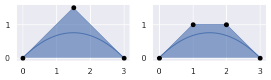

void BEZ_evaluate_curve_barycentric(const int *num_nodes, const int *dimension, const double *nodes, const int *num_vals, const double *lambda1, const double *lambda2, double *evaluated)

For a Bézier curve with control points \(p_0, \ldots, p_d\), this evaluates the quantity

\[Q(\lambda_1, \lambda_2) = \sum_{j = 0}^d \binom{d}{j} \lambda_1^{d - j} \lambda_2^j p_j.\]

The typical case is barycentric, i.e. \(\lambda_1 + \lambda_2 = 1\), but this is not required.

Parameters

• num_nodes (const int*) – [Input] The number of control points \(N\) of a Bézier curve.

• dimension (const int*) – [Input] The dimension \(D\) such that the curve lies in \(\mathbf{R}^D\).

• nodes (const double*) – [Input] The actual control points of the curve as a \(D \times N\) array. This should be laid out in Fortran order, with \(D N\) total values.

• num_vals (const int*) – [Input] The number of values \(k\) where the quantity will be evaluated.

• lambda1 (const double*) – [Input] An array of \(k\) values used for the first parameter \(\lambda_1\).

• lambda2 (const double*) – [Input] An array of \(k\) values used for the second parameter \(\lambda_2\).

• evaluated (double*) – [Output] The evaluated quantites as a \(D \times k\) array, laid out in Fortran order. Column \(j\) of evaluated will contain \(Q\left(\lambda_1\left[j\right], \lambda_2\left[j\right]\right)\).

Signature:

void
BEZ_evaluate_curve_barycentric(const int *num_nodes,
                               const int *dimension,
                               const double *nodes,
                               const int *num_vals,
                               const double *lambda1,
                               const double *lambda2,
                               double *evaluated);

Example:

For the curve \(B(s) = \left[\begin{array}{c} 0 \\ 1 \end{array}\right] (1 - s)^2 + \left[\begin{array}{c} 2 \\ 1 \end{array}\right] 2 (1 - s) s + \left[\begin{array}{c} 3 \\ 3 \end{array}\right] s^2 = \left[\begin{array}{c} s(4 - s) \\ 2s^2 + 1 \end{array}\right]\):

// Inputs.
int num_nodes = 3;
int dimension = 2;
double nodes[6] = { 0.0, 1.0, 2.0, 1.0, 3.0, 3.0 };
int num_vals = 4;
double lambda1[4] = { 0.25, 0.5, 0.0, 1.0 };
double lambda2[4] = { 0.75, 0.25, 0.5, 0.25 };

// Outputs.
double evaluated[8];

BEZ_evaluate_curve_barycentric(
    &num_nodes, &dimension, nodes, &num_vals, lambda1, lambda2, evaluated);
printf("Evaluated:\n");
printf("%f, %f, %f, %f\n", evaluated[0], evaluated[2], evaluated[4],
    evaluated[6]);
printf("%f, %f, %f, %f\n", evaluated[1], evaluated[3], evaluated[5],
    evaluated[7]);

we have

\[\begin{split}\begin{align*} Q\left(\frac{1}{4}, \frac{3}{4}\right) &= \frac{1}{16} \left[ \begin{array}{c} 39 \\ 34 \end{array}\right] \\ Q\left(\frac{1}{2}, \frac{1}{4}\right) &= \frac{1}{16} \left[ \begin{array}{c} 11 \\ 11 \end{array}\right] \\ Q\left(0, \frac{1}{2}\right) &= \frac{1}{4} \left[ \begin{array}{c} 3 \\ 3 \end{array}\right] \\ Q\left(1, \frac{1}{4}\right) &= \frac{1}{16} \left[ \begin{array}{c} 19 \\ 27 \end{array}\right] \end{align*}\end{split}\]

$ INCLUDE_DIR=.../libbezier-release/usr/include
$ LIB_DIR=.../libbezier-release/usr/lib
$ gcc \
>     -o example \
>     example_evaluate_curve_barycentric.c \
>     -I "${INCLUDE_DIR}" \
>     -L "${LIB_DIR}" \
>     -Wl,-rpath,"${LIB_DIR}" \
>     -lbezier \
>     -lm -lgfortran
$ ./example
Evaluated:
2.437500, 0.687500, 0.750000, 1.187500
2.125000, 0.687500, 0.750000, 1.687500

void BEZ_evaluate_hodograph(const double *s, const int *num_nodes, const int *dimension, const double *nodes, double *hodograph)

Evaluates the hodograph (or derivative) of a Bézier curve function \(B'(s)\).

Parameters

• s (const double*) – [Input] The parameter \(s\) where the hodograph is being computed.

• num_nodes (const int*) – [Input] The number of control points \(N\) of a Bézier curve.

• dimension (const int*) – [Input] The dimension \(D\) such that the curve lies in \(\mathbf{R}^D\).

• nodes (const double*) – [Input] The actual control points of the curve as a \(D \times N\) array. This should be laid out in Fortran order, with \(D N\) total values.

• hodograph (double*) – [Output] The hodograph \(B'(s)\) as a \(D \times 1\) array.

Signature:

void
BEZ_evaluate_hodograph(const double *s,
                       const int *num_nodes,
                       const int *dimension,
                       const double *nodes,
                       double *hodograph);

Example:

For the curve \(B(s) = \left[\begin{array}{c} 1 \\ 0 \end{array}\right] (1 - s)^3 + \left[\begin{array}{c} 1 \\ 1 \end{array}\right] 3 (1 - s)^2 s + \left[\begin{array}{c} 2 \\ 0 \end{array}\right] 3 (1 - s) s^2 + \left[\begin{array}{c} 2 \\ 1 \end{array}\right] s^3\):

// Inputs.
double s = 0.125;
int num_nodes = 4;
int dimension = 2;
double nodes[8] = { 1.0, 0.0, 1.0, 1.0, 2.0, 0.0, 2.0, 1.0 };

// Outputs.
double hodograph[2];

BEZ_evaluate_hodograph(&s, &num_nodes, &dimension, nodes, hodograph);
printf("Hodograph:\n%f\n%f\n", hodograph[0], hodograph[1]);

we have \(B'\left(\frac{1}{8}\right) = \frac{1}{32} \left[ \begin{array}{c} 21 \\ 54 \end{array}\right]\):

$ INCLUDE_DIR=.../libbezier-release/usr/include
$ LIB_DIR=.../libbezier-release/usr/lib
$ gcc \
>     -o example \
>     example_evaluate_hodograph.c \
>     -I "${INCLUDE_DIR}" \
>     -L "${LIB_DIR}" \
>     -Wl,-rpath,"${LIB_DIR}" \
>     -lbezier \
>     -lm -lgfortran
$ ./example
Hodograph:
0.656250
1.687500

void BEZ_evaluate_multi(const int *num_nodes, const int *dimension, const double *nodes, const int *num_vals, const double *s_vals, double *evaluated)

Evaluate a Bézier curve function \(B(s_j)\) at multiple values \(\left\{s_j\right\}_j\).

Parameters

• num_nodes (const int*) – [Input] The number of control points \(N\) of a Bézier curve.

• dimension (const int*) – [Input] The dimension \(D\) such that the curve lies in \(\mathbf{R}^D\).

• nodes (const double*) – [Input] The actual control points of the curve as a \(D \times N\) array. This should be laid out in Fortran order, with \(D N\) total values.

• num_vals (const int*) – [Input] The number of values \(k\) where the \(B(s)\) will be evaluated.

• s_vals (const double*) – [Input] An array of \(k\) values \(s_j\).

• evaluated (double*) – [Output] The evaluated points as a \(D \times k\) array, laid out in Fortran order. Column \(j\) of evaluated will contain \(B\left(s_j\right)\).

Signature:

void
BEZ_evaluate_multi(const int *num_nodes,
                   const int *dimension,
                   const double *nodes,
                   const int *num_vals,
                   const double *s_vals,
                   double *evaluated);

Example:

For the curve \(B(s) = \left[\begin{array}{c} 1 \\ 0 \end{array}\right] (1 - s)^3 + \left[\begin{array}{c} 1 \\ 1 \end{array}\right] 3 (1 - s)^2 s + \left[\begin{array}{c} 2 \\ 0 \end{array}\right] 3 (1 - s) s^2 + \left[\begin{array}{c} 2 \\ 1 \end{array}\right] s^3\):

// Inputs.
int num_nodes = 4;
int dimension = 2;
double nodes[8] = { 1.0, 0.0, 1.0, 1.0, 2.0, 0.0, 2.0, 1.0 };
int num_vals = 3;
double s_vals[3] = { 0.0, 0.5, 1.0 };

// Outputs.
double evaluated[6];

BEZ_evaluate_multi(
    &num_nodes, &dimension, nodes, &num_vals, s_vals, evaluated);
printf("Evaluated:\n");
printf("%f, %f, %f\n", evaluated[0], evaluated[2], evaluated[4]);
printf("%f, %f, %f\n", evaluated[1], evaluated[3], evaluated[5]);

we have \(B\left(0\right) = \left[\begin{array}{c} 1 \\ 0 \end{array}\right], B\left(\frac{1}{2}\right) = \frac{1}{2} \left[\begin{array}{c} 3 \\ 1 \end{array}\right]\) and \(B\left(1\right) = \left[\begin{array}{c} 2 \\ 1 \end{array}\right]\):

$ INCLUDE_DIR=.../libbezier-release/usr/include
$ LIB_DIR=.../libbezier-release/usr/lib
$ gcc \
>     -o example \
>     example_evaluate_multi.c \
>     -I "${INCLUDE_DIR}" \
>     -L "${LIB_DIR}" \
>     -Wl,-rpath,"${LIB_DIR}" \
>     -lbezier \
>     -lm -lgfortran
$ ./example
Evaluated:
1.000000, 1.500000, 2.000000
0.000000, 0.500000, 1.000000

void BEZ_full_reduce(const int *num_nodes, const int *dimension, const double *nodes, const int *num_reduced_nodes, double *reduced, bool *not_implemented)

Perform a “full” degree reduction. Does so by using BEZ_reduce_pseudo_inverse() continually until the degree of the curve can no longer be reduced.

Parameters

• num_nodes (const int*) – [Input] The number of control points \(N\) of a Bézier curve.

• dimension (const int*) – [Input] The dimension \(D\) such that the curve lies in \(\mathbf{R}^D\).

• nodes (const double*) – [Input] The actual control points of the curve as a \(D \times N\) array. This should be laid out in Fortran order, with \(D N\) total values.

• num_reduced_nodes (const int*) – [Output] The number of control points \(M\) of the fully reduced curve.

• reduced (double*) – [Output] The control points of the fully reduced curve as a \(D \times N\) array. The first \(M\) columns will contain the reduced nodes. reduced must be allocated by the caller and since \(M = N\) occurs when no reduction is possible, this array must be \(D \times N\).

• not_implemented (bool*) – [Output] Indicates if degree-reduction has been implemented for the current curve’s degree. (Currently, the only degrees supported are 1, 2, 3 and 4.)

Signature:

void
BEZ_full_reduce(const int *num_nodes,
                const int *dimension,
                const double *nodes,
                const int *num_reduced_nodes,
                double *reduced,
                bool *not_implemented);

Example:

When taking a curve that is degree-elevated from linear to quartic:

// Inputs.
int num_nodes = 5;
int dimension = 2;
double nodes[10] = { 1.0, 3.0, 1.25, 3.5, 1.5, 4.0, 1.75, 4.5, 2.0, 5.0 };

// Outputs.
int num_reduced_nodes;
double reduced[10];
bool not_implemented;

BEZ_full_reduce(&num_nodes, &dimension, nodes, &num_reduced_nodes, reduced,
    &not_implemented);
printf("Number of reduced nodes: %d\n", num_reduced_nodes);
printf("Reduced:\n");
printf("%f, %f\n", reduced[0], reduced[2]);
printf("%f, %f\n", reduced[1], reduced[3]);
printf("Not implemented: %s\n", not_implemented ? "TRUE" : "FALSE");

this procedure reduces it to the line \(B(s) = \left[\begin{array}{c} 1 \\ 3 \end{array}\right] (1 - s) + \left[\begin{array}{c} 2 \\ 5 \end{array}\right] s = \left[\begin{array}{c} 1 + s \\ 3 + 2s \end{array}\right]\):

$ INCLUDE_DIR=.../libbezier-release/usr/include
$ LIB_DIR=.../libbezier-release/usr/lib
$ gcc \
>     -o example \
>     example_full_reduce.c \
>     -I "${INCLUDE_DIR}" \
>     -L "${LIB_DIR}" \
>     -Wl,-rpath,"${LIB_DIR}" \
>     -lbezier \
>     -lm -lgfortran
$ ./example
Number of reduced nodes: 2
Reduced:
1.000000, 2.000000
3.000000, 5.000000
Not implemented: FALSE

void BEZ_get_curvature(const int *num_nodes, const double *nodes, const double *tangent_vec, const double *s, double *curvature)

Get the signed curvature of a Bézier curve at a point. See hazmat.curve_helpers.get_curvature() for more details.

Note

This only computes curvature for plane curves (i.e. curves in \(\mathbf{R}^2\)). An equivalent notion of curvature exists for space curves, but support for that is not implemented here.

Parameters

• num_nodes (const int*) – [Input] The number of control points \(N\) of a Bézier curve.

• nodes (const double*) – [Input] The actual control points of the curve as a \(2 \times N\) array. This should be laid out in Fortran order, with \(2 N\) total values.

• tangent_vec (const double*) – [Input] The hodograph \(B'(s)\) as a \(2 \times 1\) array. Note that this could be computed once \(s\) and \(B\) are known, but this allows the caller to re-use an already computed tangent vector.

• s (const double*) – [Input] The parameter \(s\) where the curvature is being computed.

• curvature (double*) – [Output] The signed curvature \(\kappa\).

Signature:

void
BEZ_get_curvature(const int *num_nodes,
                  const double *nodes,
                  const double *tangent_vec,
                  const double *s,
                  double *curvature);

Example:

// Inputs.
int num_nodes = 5;
double nodes[10] = { 1.0, 0.0, 0.75, 2.0, 0.5, -2.0, 0.25, 2.0, 0.0, 0.0 };
double tangent_vec[2] = { -1.0, 0.0 };
double s = 0.5;

// Outputs.
double curvature;

BEZ_get_curvature(&num_nodes, nodes, tangent_vec, &s, &curvature);
printf("Curvature: %f\n", curvature);

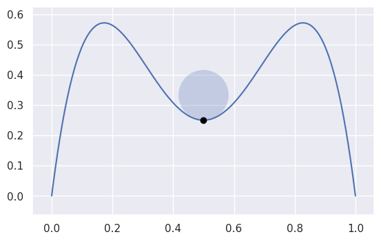
$ INCLUDE_DIR=.../libbezier-release/usr/include
$ LIB_DIR=.../libbezier-release/usr/lib
$ gcc \
>     -o example \
>     example_get_curvature.c \
>     -I "${INCLUDE_DIR}" \
>     -L "${LIB_DIR}" \
>     -Wl,-rpath,"${LIB_DIR}" \
>     -lbezier \
>     -lm -lgfortran
$ ./example
Curvature: -12.000000

void BEZ_locate_point_curve(const int *num_nodes, const int *dimension, const double *nodes, const double *point, double *s_approx)

This solves the inverse problem \(B(s) = p\) (if it can be solved). Does so by subdividing the curve until the segments are sufficiently small, then using Newton’s method to narrow in on the pre-image of the point.

Parameters

• num_nodes (const int*) – [Input] The number of control points \(N\) of a Bézier curve.

• dimension (const int*) – [Input] The dimension \(D\) such that the curve lies in \(\mathbf{R}^D\).

• nodes (const double*) – [Input] The actual control points of the curve as a \(D \times N\) array. This should be laid out in Fortran order, with \(D N\) total values.

• point (const double*) – [Input] The point \(p\) as a \(D \times 1\) array.

• s_approx (double*) – [Output] The parameter \(s\) of the solution. If \(p\) can’t be located on the curve, then s_approx = -1.0. If there are multiple parameters that satisfy \(B(s) = p\) (indicating that \(B(s)\) has a self-crossing) then s_approx = -2.0.

Signature:

void
BEZ_locate_point_curve(const int *num_nodes,
                       const int *dimension,
                       const double *nodes,
                       const double *point,
                       double *s_approx);

Example:

For \(B(s) = \left[\begin{array}{c} 0 \\ 2 \end{array}\right] (1 - s)^3 + \left[\begin{array}{c} -1 \\ 0 \end{array}\right] 3 (1 - s)^2 s + \left[\begin{array}{c} 1 \\ 1 \end{array}\right] 3 (1 - s) s^2 + \frac{1}{8} \left[\begin{array}{c} -6 \\ 13 \end{array}\right] s^3\):

// Inputs.
int num_nodes = 4;
int dimension = 2;
double nodes[8] = { 0.0, 2.0, -1.0, 0.0, 1.0, 1.0, -0.75, 1.625 };
double point1[2] = { -0.09375, 0.828125 };
double point2[2] = { 0.0, 1.5 };
double point3[2] = { -0.25, 1.375 };

// Outputs.
double s_approx;

BEZ_locate_point_curve(&num_nodes, &dimension, nodes, point1, &s_approx);
printf("When B(s) = [% f, %f]; s = % f\n", point1[0], point1[1], s_approx);
BEZ_locate_point_curve(&num_nodes, &dimension, nodes, point2, &s_approx);
printf("When B(s) = [% f, %f]; s = % f\n", point2[0], point2[1], s_approx);
BEZ_locate_point_curve(&num_nodes, &dimension, nodes, point3, &s_approx);
printf("When B(s) = [% f, %f]; s = % f\n", point3[0], point3[1], s_approx);

We can locate the point \(B\left(\frac{1}{2}\right) = \frac{1}{64} \left[\begin{array}{c} -6 \\ 53 \end{array}\right]\) but find that \(\frac{1}{2} \left[\begin{array}{c} 0 \\ 3 \end{array}\right]\) is not on the curve and that

\[\begin{split}B\left(\frac{3 - \sqrt{5}}{6}\right) = B\left(\frac{3 + \sqrt{5}}{6}\right) = \frac{1}{8} \left[ \begin{array}{c} -2 \\ 11 \end{array}\right]\end{split}\]

is a self-crossing:

$ INCLUDE_DIR=.../libbezier-release/usr/include
$ LIB_DIR=.../libbezier-release/usr/lib
$ gcc \
>     -o example \
>     example_locate_point_curve.c \
>     -I "${INCLUDE_DIR}" \
>     -L "${LIB_DIR}" \
>     -Wl,-rpath,"${LIB_DIR}" \
>     -lbezier \
>     -lm -lgfortran
$ ./example
When B(s) = [-0.093750, 0.828125]; s =  0.500000
When B(s) = [ 0.000000, 1.500000]; s = -1.000000
When B(s) = [-0.250000, 1.375000]; s = -2.000000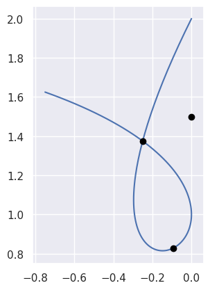

void BEZ_newton_refine_curve(const int *num_nodes, const int *dimension, const double *nodes, const double *point, const double *s, double *updated_s)

This refines a solution to \(B(s) = p\) using Newton’s method. Given a current approximation \(s_n\) for a solution, this produces the updated approximation via

\[s_{n + 1} = s_n - \frac{B'(s_n)^T \left[B(s_n) - p\right]}{ B'(s_n)^T B'(s_n)}.\]

Parameters

• num_nodes (const int*) – [Input] The number of control points \(N\) of a Bézier curve.

• dimension (const int*) – [Input] The dimension \(D\) such that the curve lies in \(\mathbf{R}^D\).

• nodes (const double*) – [Input] The actual control points of the curve as a \(D \times N\) array. This should be laid out in Fortran order, with \(D N\) total values.

• point (const double*) – [Input] The point \(p\) as a \(D \times 1\) array.

• s (const double*) – [Input] The parameter \(s_n\) of the current approximation of a solution.

• updated_s (double*) – [Output] The parameter \(s_{n + 1}\) of the updated approximation.

Signature:

void
BEZ_newton_refine_curve(const int *num_nodes,
                        const int *dimension,
                        const double *nodes,
                        const double *point,
                        const double *s,
                        double *updated_s);

Example:

When trying to locate \(B\left(\frac{1}{4}\right) = \frac{1}{16} \left[\begin{array}{c} 9 \\ 13 \end{array}\right]\) on the curve \(B(s) = \left[\begin{array}{c} 0 \\ 0 \end{array}\right] (1 - s)^2 + \left[\begin{array}{c} 1 \\ 2 \end{array}\right] 2 (1 - s) s + \left[\begin{array}{c} 3 \\ 1 \end{array}\right] s^2\), starting at \(s = \frac{3}{4}\):

// Inputs.
int num_nodes = 3;
int dimension = 2;
double nodes[6] = { 0.0, 0.0, 1.0, 2.0, 3.0, 1.0 };
double point[2] = { 0.5625, 0.8125 };
double s = 0.75;

// Outputs.
double updated_s;

BEZ_newton_refine_curve(
    &num_nodes, &dimension, nodes, point, &s, &updated_s);

we expect a Newton update \(\Delta s = -\frac{2}{5}\), which produces a new parameter value \(s = \frac{7}{20}\):

$ INCLUDE_DIR=.../libbezier-release/usr/include
$ LIB_DIR=.../libbezier-release/usr/lib
$ gcc \
>     -o example \
>     example_newton_refine_curve.c \
>     -I "${INCLUDE_DIR}" \
>     -L "${LIB_DIR}" \
>     -Wl,-rpath,"${LIB_DIR}" \
>     -lbezier \
>     -lm -lgfortran
$ ./example
Updated s: 0.350000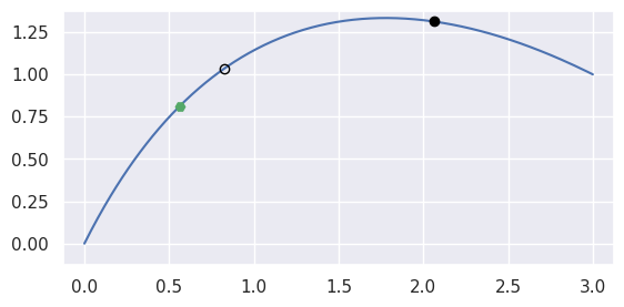

void BEZ_reduce_pseudo_inverse(const int *num_nodes, const int *dimension, const double *nodes, double *reduced, bool *not_implemented)

Perform a pseudo inverse to BEZ_elevate_nodes_curve(). If an inverse can be found, i.e. if a curve can be degree-reduced, then this will produce the equivalent curve of lower degree. If no inverse can be found, then this will produce the “best” answer in the least squares sense.

Parameters

• num_nodes (const int*) – [Input] The number of control points \(N\) of a Bézier curve.

• dimension (const int*) – [Input] The dimension \(D\) such that the curve lies in \(\mathbf{R}^D\).

• nodes (const double*) – [Input] The actual control points of the curve as a \(D \times N\) array. This should be laid out in Fortran order, with \(D N\) total values.

• reduced (double*) – [Output] The control points of the degree-(pseudo)reduced curve \(D \times (N - 1)\) array, laid out in Fortran order.

• not_implemented (bool*) – [Output] Indicates if degree-reduction has been implemented for the current curve’s degree. (Currently, the only degrees supported are 1, 2, 3 and 4.)

Signature:

void
BEZ_reduce_pseudo_inverse(const int *num_nodes,
                          const int *dimension,
                          const double *nodes,
                          double *reduced,
                          bool *not_implemented);

Example:

After reducing \(B(s) = \left[\begin{array}{c} -3 \\ 3 \end{array}\right] (1 - s)^3 + \left[\begin{array}{c} 0 \\ 2 \end{array}\right] 3 (1 - s)^2 s + \left[\begin{array}{c} 1 \\ 3 \end{array}\right] 3 (1 - s) s^2 + \left[\begin{array}{c} 0 \\ 6 \end{array}\right] s^3\):

// Inputs.
int num_nodes = 4;
int dimension = 2;
double nodes[8] = { -3.0, 3.0, 0.0, 2.0, 1.0, 3.0, 0.0, 6.0 };

// Outputs.
double reduced[6];
bool not_implemented;

BEZ_reduce_pseudo_inverse(
    &num_nodes, &dimension, nodes, reduced, &not_implemented);
printf("Reduced:\n");
printf("% f, %f, %f\n", reduced[0], reduced[2], reduced[4]);
printf("% f, %f, %f\n", reduced[1], reduced[3], reduced[5]);
printf("Not implemented: %s\n", not_implemented ? "TRUE" : "FALSE");

we get the valid quadratic representation of \(B(s) = \left[\begin{array}{c} 3(1 - s)(2s - 1) \\ 3(2s^2 - s + 1) \end{array}\right]\):

$ INCLUDE_DIR=.../libbezier-release/usr/include
$ LIB_DIR=.../libbezier-release/usr/lib
$ gcc \
>     -o example \
>     example_reduce_pseudo_inverse.c \
>     -I "${INCLUDE_DIR}" \
>     -L "${LIB_DIR}" \
>     -Wl,-rpath,"${LIB_DIR}" \
>     -lbezier \
>     -lm -lgfortran
$ ./example
Reduced:
-3.000000, 1.500000, 0.000000
 3.000000, 1.500000, 6.000000
Not implemented: FALSE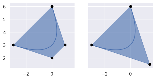

void BEZ_specialize_curve(const int *num_nodes, const int *dimension, const double *nodes, const double *start, const double *end, double *new_nodes)

Specialize a Bézier curve to an interval \(\left[a, b\right]\). This produces the control points for the curve given by \(B\left(a + (b - a) s\right)\).

Parameters

• num_nodes (const int*) – [Input] The number of control points \(N\) of a Bézier curve.

• dimension (const int*) – [Input] The dimension \(D\) such that the curve lies in \(\mathbf{R}^D\).

• nodes (const double*) – [Input] The actual control points of the curve as a \(D \times N\) array. This should be laid out in Fortran order, with \(D N\) total values.

• start (const double*) – [Input] The start \(a\) of the specialized interval.

• end (const double*) – [Input] The end \(b\) of the specialized interval.

• new_nodes (double*) – [Output] The control points of the specialized curve, as a \(D \times N\) array, laid out in Fortran order.

Signature:

void
BEZ_specialize_curve(const int *num_nodes,
                     const int *dimension,
                     const double *nodes,
                     const double *start,
                     const double *end,
                     double *new_nodes);

Example:

When we specialize the curve \(B(s) = \left[\begin{array}{c} 0 \\ 0 \end{array}\right] (1 - s)^2 + \frac{1}{2} \left[\begin{array}{c} 1 \\ 2 \end{array}\right] 2 (1 - s) s + \left[\begin{array}{c} 1 \\ 0 \end{array}\right] s^2 = \left[\begin{array}{c} s \\ 2s(1 - s) \end{array}\right]\) to the interval \(\left[-\frac{1}{4}, \frac{3}{4}\right]\):

// Inputs.
int num_nodes = 3;
int dimension = 2;
double nodes[6] = { 0.0, 0.0, 0.5, 1.0, 1.0, 0.0 };
double start = -0.25;
double end = 0.75;

// Outputs.
double new_nodes[6];

BEZ_specialize_curve(
    &num_nodes, &dimension, nodes, &start, &end, new_nodes);
printf("New Nodes:\n");
printf("%f, %f, %f\n", new_nodes[0], new_nodes[2], new_nodes[4]);

we get the specialized curve \(S(t) = \frac{1}{8} \left[ \begin{array}{c} -2 \\ -5 \end{array}\right] (1 - s)^2 + \frac{1}{8} \left[\begin{array}{c} 2 \\ 7 \end{array}\right] 2 (1 - s) s + \frac{1}{8} \left[\begin{array}{c} 6 \\ 3 \end{array}\right] s^2 = \frac{1}{8} \left[\begin{array}{c} 2(4t - 1) \\ (4t - 1)(5 - 4t) \end{array}\right]\), which still lies on \(y = 2x(1 - x)\):

$ INCLUDE_DIR=.../libbezier-release/usr/include
$ LIB_DIR=.../libbezier-release/usr/lib
$ gcc \
>     -o example \
>     example_specialize_curve.c \
>     -I "${INCLUDE_DIR}" \
>     -L "${LIB_DIR}" \
>     -Wl,-rpath,"${LIB_DIR}" \
>     -lbezier \
>     -lm -lgfortran
$ ./example
New Nodes:
-0.250000, 0.250000, 0.750000
-0.625000, 0.875000, 0.375000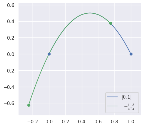

void BEZ_subdivide_nodes_curve(const int *num_nodes, const int *dimension, const double *nodes, double *left_nodes, double *right_nodes)

Split a Bézier curve into two halves \(B\left(\left[0, \frac{1}{2}\right]\right)\) and \(B\left(\left[\frac{1}{2}, 1\right]\right)\).

Parameters

• num_nodes (const int*) – [Input] The number of control points \(N\) of a Bézier curve.

• dimension (const int*) – [Input] The dimension \(D\) such that the curve lies in \(\mathbf{R}^D\).

• nodes (const double*) – [Input] The actual control points of the curve as a \(D \times N\) array. This should be laid out in Fortran order, with \(D N\) total values.

• left_nodes (double*) – [Output] The control points of the left half curve \(B\left(\left[0, \frac{1}{2}\right]\right)\) as a \(D \times N\) array, laid out in Fortran order.

• right_nodes (double*) – [Output] The control points of the right half curve \(B\left(\left[\frac{1}{2}, 1\right]\right)\) as a \(D \times N\) array, laid out in Fortran order.

Signature:

void
BEZ_subdivide_nodes_curve(const int *num_nodes,
                          const int *dimension,
                          const double *nodes,
                          double *left_nodes,
                          double *right_nodes);

Example:

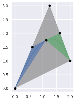
For example, subdividing the curve \(B(s) = \left[\begin{array}{c} 0 \\ 0 \end{array}\right] (1 - s)^2 + \frac{1}{4} \left[\begin{array}{c} 5 \\ 12 \end{array}\right] 2 (1 - s) s + \left[\begin{array}{c} 2 \\ 1 \end{array}\right] s^2\):

// Inputs.
int num_nodes = 3;
int dimension = 2;
double nodes[6] = { 0.0, 0.0, 1.25, 3.0, 2.0, 1.0 };

// Outputs.
double left_nodes[6];
double right_nodes[6];

BEZ_subdivide_nodes_curve(
    &num_nodes, &dimension, nodes, left_nodes, right_nodes);
printf("Left Nodes:\n");
printf("%f, %f, %f\n", left_nodes[0], left_nodes[2], left_nodes[4]);
printf("%f, %f, %f\n", left_nodes[1], left_nodes[3], left_nodes[5]);
printf("Right Nodes:\n");
printf("%f, %f, %f\n", right_nodes[0], right_nodes[2], right_nodes[4]);
printf("%f, %f, %f\n", right_nodes[1], right_nodes[3], right_nodes[5]);

yields:

$ INCLUDE_DIR=.../libbezier-release/usr/include
$ LIB_DIR=.../libbezier-release/usr/lib
$ gcc \
>     -o example \
>     example_subdivide_nodes_curve.c \
>     -I "${INCLUDE_DIR}" \
>     -L "${LIB_DIR}" \
>     -Wl,-rpath,"${LIB_DIR}" \
>     -lbezier \
>     -lm -lgfortran
$ ./example
Left Nodes:
0.000000, 0.625000, 1.125000
0.000000, 1.500000, 1.750000
Right Nodes:
1.125000, 1.625000, 2.000000
1.750000, 2.000000, 1.000000