Geometric Helpers
Functions
-
bezier._py_intersection_helpers.newton_refine(s, nodes1, t, nodes2)¶ Apply one step of 2D Newton’s method.
Note
There is also a Fortran implementation of this function, which will be used if it can be built.
We want to use Newton’s method on the function
\[F(s, t) = B_1(s) - B_2(t)\]to refine \(\left(s_{\ast}, t_{\ast}\right)\). Using this, and the Jacobian \(DF\), we “solve”
\[\begin{split}\left[\begin{array}{c} 0 \\ 0 \end{array}\right] \approx F\left(s_{\ast} + \Delta s, t_{\ast} + \Delta t\right) \approx F\left(s_{\ast}, t_{\ast}\right) + \left[\begin{array}{c c} B_1'\left(s_{\ast}\right) & - B_2'\left(t_{\ast}\right) \end{array}\right] \left[\begin{array}{c} \Delta s \\ \Delta t \end{array}\right]\end{split}\]and refine with the component updates \(\Delta s\) and \(\Delta t\).
Note
This implementation assumes the curves live in \(\mathbf{R}^2\).
For example, the curves
\[\begin{split}\begin{align*} B_1(s) &= \left[\begin{array}{c} 0 \\ 0 \end{array}\right] (1 - s)^2 + \left[\begin{array}{c} 2 \\ 4 \end{array}\right] 2s(1 - s) + \left[\begin{array}{c} 4 \\ 0 \end{array}\right] s^2 \\ B_2(t) &= \left[\begin{array}{c} 2 \\ 0 \end{array}\right] (1 - t) + \left[\begin{array}{c} 0 \\ 3 \end{array}\right] t \end{align*}\end{split}\]intersect at the point \(B_1\left(\frac{1}{4}\right) = B_2\left(\frac{1}{2}\right) = \frac{1}{2} \left[\begin{array}{c} 2 \\ 3 \end{array}\right]\).
However, starting from the wrong point we have
\[\begin{split}\begin{align*} F\left(\frac{3}{8}, \frac{1}{4}\right) &= \frac{1}{8} \left[\begin{array}{c} 0 \\ 9 \end{array}\right] \\ DF\left(\frac{3}{8}, \frac{1}{4}\right) &= \left[\begin{array}{c c} 4 & 2 \\ 2 & -3 \end{array}\right] \\ \Longrightarrow \left[\begin{array}{c} \Delta s \\ \Delta t \end{array}\right] &= \frac{9}{64} \left[\begin{array}{c} -1 \\ 2 \end{array}\right]. \end{align*}\end{split}\]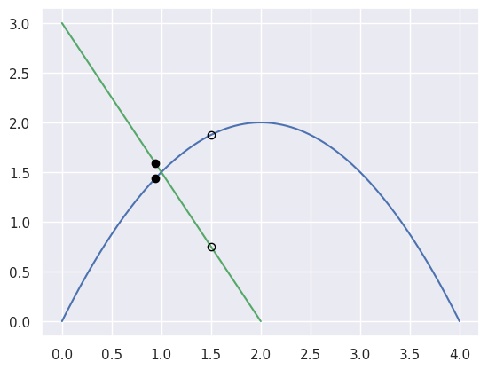
>>> nodes1 = np.asfortranarray([
...     [0.0, 2.0, 4.0],
...     [0.0, 4.0, 0.0],
... ])
>>> nodes2 = np.asfortranarray([
...     [2.0, 0.0],
...     [0.0, 3.0],
... ])
>>> s, t = 0.375, 0.25
>>> new_s, new_t = newton_refine(s, nodes1, t, nodes2)
>>> 64.0 * (new_s - s)
-9.0
>>> 64.0 * (new_t - t)
18.0
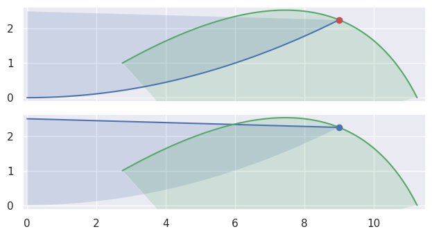
For “typical” curves, we converge to a solution quadratically. This means that the number of correct digits doubles every iteration (until machine precision is reached).
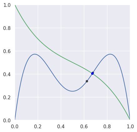
>>> nodes1 = np.asfortranarray([
...     [0.0, 0.25,  0.5, 0.75, 1.0],
...     [0.0, 2.0 , -2.0, 2.0 , 0.0],
... ])
>>> nodes2 = np.asfortranarray([
...     [0.0, 0.25, 0.5, 0.75, 1.0],
...     [1.0, 0.5 , 0.5, 0.5 , 0.0],
... ])
>>> # The expected intersection is the only real root of
>>> # 28 s^3 - 30 s^2 + 9 s - 1.
>>> expected, = realroots(28, -30, 9, -1)
>>> s_vals = [0.625, None, None, None, None]
>>> t = 0.625
>>> np.log2(abs(expected - s_vals[0]))
-4.399...
>>> s_vals[1], t = newton_refine(s_vals[0], nodes1, t, nodes2)
>>> np.log2(abs(expected - s_vals[1]))
-7.901...
>>> s_vals[2], t = newton_refine(s_vals[1], nodes1, t, nodes2)
>>> np.log2(abs(expected - s_vals[2]))
-16.010...
>>> s_vals[3], t = newton_refine(s_vals[2], nodes1, t, nodes2)
>>> np.log2(abs(expected - s_vals[3]))
-32.110...
>>> s_vals[4], t = newton_refine(s_vals[3], nodes1, t, nodes2)
>>> np.allclose(s_vals[4], expected, rtol=6 * machine_eps, atol=0.0)
True
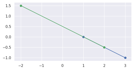
However, when the intersection occurs at a point of tangency, the convergence becomes linear. This means that the number of correct digits added each iteration is roughly constant.
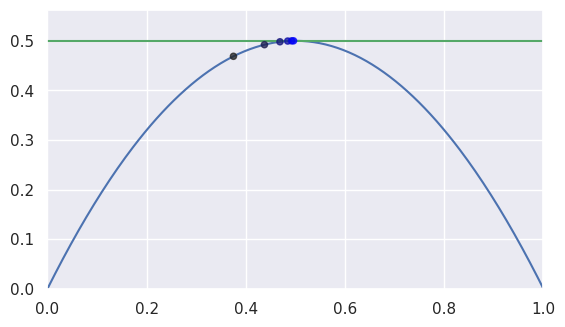
>>> nodes1 = np.asfortranarray([
...     [0.0, 0.5, 1.0],
...     [0.0, 1.0, 0.0],
... ])
>>> nodes2 = np.asfortranarray([
...     [0.0, 1.0],
...     [0.5, 0.5],
... ])
>>> expected = 0.5
>>> s_vals = [0.375, None, None, None, None, None]
>>> t = 0.375
>>> np.log2(abs(expected - s_vals[0]))
-3.0
>>> s_vals[1], t = newton_refine(s_vals[0], nodes1, t, nodes2)
>>> np.log2(abs(expected - s_vals[1]))
-4.0
>>> s_vals[2], t = newton_refine(s_vals[1], nodes1, t, nodes2)
>>> np.log2(abs(expected - s_vals[2]))
-5.0
>>> s_vals[3], t = newton_refine(s_vals[2], nodes1, t, nodes2)
>>> np.log2(abs(expected - s_vals[3]))
-6.0
>>> s_vals[4], t = newton_refine(s_vals[3], nodes1, t, nodes2)
>>> np.log2(abs(expected - s_vals[4]))
-7.0
>>> s_vals[5], t = newton_refine(s_vals[4], nodes1, t, nodes2)
>>> np.log2(abs(expected - s_vals[5]))
-8.0
Unfortunately, the process terminates with an error that is not close to machine precision \(\varepsilon\) when \(\Delta s = \Delta t = 0\).
>>> s1 = t1 = 0.5 - 0.5**27
>>> np.log2(0.5 - s1)
-27.0
>>> s2, t2 = newton_refine(s1, nodes1, t1, nodes2)
>>> s2 == t2
True
>>> np.log2(0.5 - s2)
-28.0
>>> s3, t3 = newton_refine(s2, nodes1, t2, nodes2)
>>> s3 == t3 == s2
True
Due to round-off near the point of tangency, the final error resembles \(\sqrt{\varepsilon}\) rather than machine precision as expected.
Note
The following is not implemented in this function. It’s just an exploration on how the shortcomings might be addressed.
However, this can be overcome. At the point of tangency, we want \(B_1'(s) \parallel B_2'(t)\). This can be checked numerically via
\[B_1'(s) \times B_2'(t) = 0.\]For the last example (the one that converges linearly), this is
\[\begin{split}0 = \left[\begin{array}{c} 1 \\ 2 - 4s \end{array}\right] \times \left[\begin{array}{c} 1 \\ 0 \end{array}\right] = 4 s - 2.\end{split}\]With this, we can modify Newton’s method to find a zero of the over-determined system
\[\begin{split}G(s, t) = \left[\begin{array}{c} B_0(s) - B_1(t) \\ B_1'(s) \times B_2'(t) \end{array}\right] = \left[\begin{array}{c} s - t \\ 2 s (1 - s) - \frac{1}{2} \\ 4 s - 2\end{array}\right].\end{split}\]Since \(DG\) is \(3 \times 2\), we can’t invert it. However, we can find a least-squares solution:
\[\begin{split}\left(DG^T DG\right) \left[\begin{array}{c} \Delta s \\ \Delta t \end{array}\right] = -DG^T G.\end{split}\]This only works if \(DG\) has full rank. In this case, it does since the submatrix containing the first and last rows has rank two:
\[\begin{split}DG = \left[\begin{array}{c c} 1 & -1 \\ 2 - 4 s & 0 \\ 4 & 0 \end{array}\right].\end{split}\]Though this avoids a singular system, the normal equations have a condition number that is the square of the condition number of the matrix.
Starting from \(s = t = \frac{3}{8}\) as above:
>>> s0, t0 = 0.375, 0.375
>>> np.log2(0.5 - s0)
-3.0
>>> s1, t1 = modified_update(s0, t0)
>>> s1 == t1
True
>>> 1040.0 * s1
519.0
>>> np.log2(0.5 - s1)
-10.022...
>>> s2, t2 = modified_update(s1, t1)
>>> s2 == t2
True
>>> np.log2(0.5 - s2)
-31.067...
>>> s3, t3 = modified_update(s2, t2)
>>> s3 == t3 == 0.5
True
- Parameters
s (float) – Parameter of a near-intersection along the first curve.
nodes1 (numpy.ndarray) – Nodes of first curve forming intersection.
t (float) – Parameter of a near-intersection along the second curve.
nodes2 (numpy.ndarray) – Nodes of second curve forming intersection.
- Returns
The refined parameters from a single Newton step.
- Return type
- Raises
ValueError – If the Jacobian is singular at
(s, t).
-
bezier._py_geometric_intersection.linearization_error(nodes)¶ Compute the maximum error of a linear approximation.
Note
There is also a Fortran implementation of this function, which will be used if it can be built.
Note
This is a helper for
Linearization, which is used during the curve-curve intersection process.We use the line
\[L(s) = v_0 (1 - s) + v_n s\]and compute a bound on the maximum error
\[\max_{s \in \left[0, 1\right]} \|B(s) - L(s)\|_2.\]Rather than computing the actual maximum (a tight bound), we use an upper bound via the remainder from Lagrange interpolation in each component. This leaves us with \(\frac{s(s - 1)}{2!}\) times the second derivative in each component.
The second derivative curve is degree \(d = n - 2\) and is given by
\[B''(s) = n(n - 1) \sum_{j = 0}^{d} \binom{d}{j} s^j (1 - s)^{d - j} \cdot \Delta^2 v_j\]Due to this form (and the convex combination property of Bézier Curves) we know each component of the second derivative will be bounded by the maximum of that component among the \(\Delta^2 v_j\).
For example, the curve
\[\begin{split}B(s) = \left[\begin{array}{c} 0 \\ 0 \end{array}\right] (1 - s)^2 + \left[\begin{array}{c} 3 \\ 1 \end{array}\right] 2s(1 - s) + \left[\begin{array}{c} 9 \\ -2 \end{array}\right] s^2\end{split}\]has \(B''(s) \equiv \left[\begin{array}{c} 6 \\ -8 \end{array}\right]\) which has norm \(10\) everywhere, hence the maximum error is
\[\left.\frac{s(1 - s)}{2!} \cdot 10\right|_{s = \frac{1}{2}} = \frac{5}{4}.\]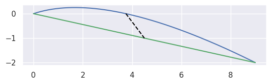
>>> nodes = np.asfortranarray([
...     [0.0, 3.0, 9.0],
...     [0.0, 1.0, -2.0],
... ])
>>> linearization_error(nodes)
1.25
As a non-example, consider a “pathological” set of control points:
\[\begin{split}B(s) = \left[\begin{array}{c} 0 \\ 0 \end{array}\right] (1 - s)^3 + \left[\begin{array}{c} 5 \\ 12 \end{array}\right] 3s(1 - s)^2 + \left[\begin{array}{c} 10 \\ 24 \end{array}\right] 3s^2(1 - s) + \left[\begin{array}{c} 30 \\ 72 \end{array}\right] s^3\end{split}\]By construction, this lies on the line \(y = \frac{12x}{5}\), but the parametrization is cubic: \(12 \cdot x(s) = 5 \cdot y(s) = 180s(s^2 + 1)\). Hence, the fact that the curve is a line is not accounted for and we take the worse case among the nodes in:
\[\begin{split}B''(s) = 3 \cdot 2 \cdot \left( \left[\begin{array}{c} 0 \\ 0 \end{array}\right] (1 - s) + \left[\begin{array}{c} 15 \\ 36 \end{array}\right] s\right)\end{split}\]which gives a nonzero maximum error:
>>> nodes = np.asfortranarray([
...     [0.0, 5.0, 10.0, 30.0],
...     [0.0, 12.0, 24.0, 72.0],
... ])
>>> linearization_error(nodes)
29.25
Though it may seem that
0is a more appropriate answer, consider the goal of this function. We seek to linearize curves and then intersect the linear approximations. Then the \(s\)-values from the line-line intersection is lifted back to the curves. Thus the error \(\|B(s) - L(s)\|_2\) is more relevant than the underyling algebraic curve containing \(B(s)\).Note
It may be more appropriate to use a relative linearization error rather than the absolute error provided here. It’s unclear if the domain \(\left[0, 1\right]\) means the error is already adequately scaled or if the error should be scaled by the arc length of the curve or the (easier-to-compute) length of the line.
- Parameters
nodes (numpy.ndarray) – Nodes of a curve.
- Returns
The maximum error between the curve and the linear approximation.
- Return type
-
bezier._py_geometric_intersection.segment_intersection(start0, end0, start1, end1)¶ Determine the intersection of two line segments.
Assumes each line is parametric
\[\begin{split}\begin{alignat*}{2} L_0(s) &= S_0 (1 - s) + E_0 s &&= S_0 + s \Delta_0 \\ L_1(t) &= S_1 (1 - t) + E_1 t &&= S_1 + t \Delta_1. \end{alignat*}\end{split}\]To solve \(S_0 + s \Delta_0 = S_1 + t \Delta_1\), we use the cross product:
\[\left(S_0 + s \Delta_0\right) \times \Delta_1 = \left(S_1 + t \Delta_1\right) \times \Delta_1 \Longrightarrow s \left(\Delta_0 \times \Delta_1\right) = \left(S_1 - S_0\right) \times \Delta_1.\]Similarly
\[\Delta_0 \times \left(S_0 + s \Delta_0\right) = \Delta_0 \times \left(S_1 + t \Delta_1\right) \Longrightarrow \left(S_1 - S_0\right) \times \Delta_0 = \Delta_0 \times \left(S_0 - S_1\right) = t \left(\Delta_0 \times \Delta_1\right).\]Note
Since our points are in \(\mathbf{R}^2\), the “traditional” cross product in \(\mathbf{R}^3\) will always point in the \(z\) direction, so in the above we mean the \(z\) component of the cross product, rather than the entire vector.
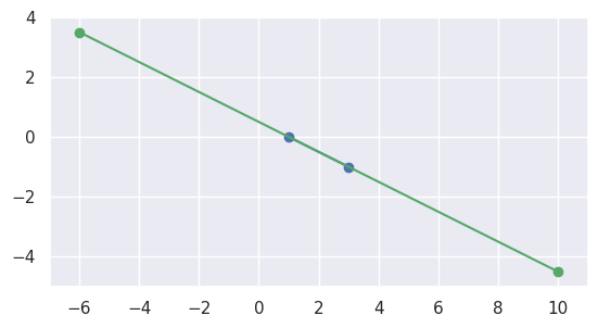
For example, the diagonal lines
\[\begin{split}\begin{align*} L_0(s) &= \left[\begin{array}{c} 0 \\ 0 \end{array}\right] (1 - s) + \left[\begin{array}{c} 2 \\ 2 \end{array}\right] s \\ L_1(t) &= \left[\begin{array}{c} -1 \\ 2 \end{array}\right] (1 - t) + \left[\begin{array}{c} 1 \\ 0 \end{array}\right] t \end{align*}\end{split}\]intersect at \(L_0\left(\frac{1}{4}\right) = L_1\left(\frac{3}{4}\right) = \frac{1}{2} \left[\begin{array}{c} 1 \\ 1 \end{array}\right]\).
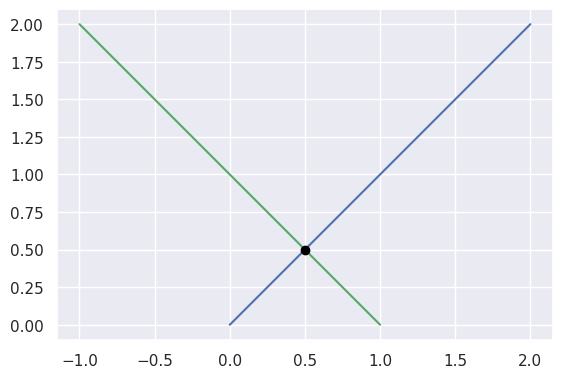
>>> start0 = np.asfortranarray([0.0, 0.0])
>>> end0 = np.asfortranarray([2.0, 2.0])
>>> start1 = np.asfortranarray([-1.0, 2.0])
>>> end1 = np.asfortranarray([1.0, 0.0])
>>> s, t, _ = segment_intersection(start0, end0, start1, end1)
>>> s
0.25
>>> t
0.75
Taking the parallel (but different) lines
\[\begin{split}\begin{align*} L_0(s) &= \left[\begin{array}{c} 1 \\ 0 \end{array}\right] (1 - s) + \left[\begin{array}{c} 0 \\ 1 \end{array}\right] s \\ L_1(t) &= \left[\begin{array}{c} -1 \\ 3 \end{array}\right] (1 - t) + \left[\begin{array}{c} 3 \\ -1 \end{array}\right] t \end{align*}\end{split}\]we should be able to determine that the lines don’t intersect, but this function is not meant for that check:
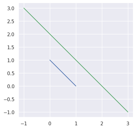
>>> start0 = np.asfortranarray([1.0, 0.0])
>>> end0 = np.asfortranarray([0.0, 1.0])
>>> start1 = np.asfortranarray([-1.0, 3.0])
>>> end1 = np.asfortranarray([3.0, -1.0])
>>> _, _, success = segment_intersection(start0, end0, start1, end1)
>>> success
False
Instead, we use
parallel_lines_parameters():>>> disjoint, _ = parallel_lines_parameters(start0, end0, start1, end1) >>> disjoint True
Note
There is also a Fortran implementation of this function, which will be used if it can be built.
- Parameters
start0 (numpy.ndarray) – A 1D NumPy
2-array that is the start vector \(S_0\) of the parametric line \(L_0(s)\).end0 (numpy.ndarray) – A 1D NumPy
2-array that is the end vector \(E_0\) of the parametric line \(L_0(s)\).start1 (numpy.ndarray) – A 1D NumPy
2-array that is the start vector \(S_1\) of the parametric line \(L_1(s)\).end1 (numpy.ndarray) – A 1D NumPy
2-array that is the end vector \(E_1\) of the parametric line \(L_1(s)\).
- Returns
Pair of \(s_{\ast}\) and \(t_{\ast}\) such that the lines intersect: \(L_0\left(s_{\ast}\right) = L_1\left(t_{\ast}\right)\) and then a boolean indicating if an intersection was found (i.e. if the lines aren’t parallel).
- Return type
-
bezier._py_geometric_intersection.parallel_lines_parameters(start0, end0, start1, end1)¶ Checks if two parallel lines ever meet.
Meant as a back-up when
segment_intersection()fails.Note
This function assumes but never verifies that the lines are parallel.
In the case that the segments are parallel and lie on different lines, then there is a guarantee of no intersection. However, if they are on the exact same line, they may define a shared segment coincident to both lines.
In
segment_intersection(), we utilized the normal form of the lines (via the cross product):\[\begin{split}\begin{align*} L_0(s) \times \Delta_0 &\equiv S_0 \times \Delta_0 \\ L_1(t) \times \Delta_1 &\equiv S_1 \times \Delta_1 \end{align*}\end{split}\]So, we can detect if \(S_1\) is on the first line by checking if
\[S_0 \times \Delta_0 \stackrel{?}{=} S_1 \times \Delta_0.\]If it is not on the first line, then we are done, the segments don’t meet:
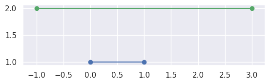
>>> # Line: y = 1
>>> start0 = np.asfortranarray([0.0, 1.0])
>>> end0 = np.asfortranarray([1.0, 1.0])
>>> # Vertical shift up: y = 2
>>> start1 = np.asfortranarray([-1.0, 2.0])
>>> end1 = np.asfortranarray([3.0, 2.0])
>>> disjoint, _ = parallel_lines_parameters(start0, end0, start1, end1)
>>> disjoint
True
If \(S_1\) is on the first line, we want to check that \(S_1\) and \(E_1\) define parameters outside of \(\left[0, 1\right]\). To compute these parameters:
\[L_1(t) = S_0 + s_{\ast} \Delta_0 \Longrightarrow s_{\ast} = \frac{\Delta_0^T \left( L_1(t) - S_0\right)}{\Delta_0^T \Delta_0}.\]For example, the intervals \(\left[0, 1\right]\) and \(\left[\frac{3}{2}, 2\right]\) (via \(S_1 = S_0 + \frac{3}{2} \Delta_0\) and \(E_1 = S_0 + 2 \Delta_0\)) correspond to segments that don’t meet:
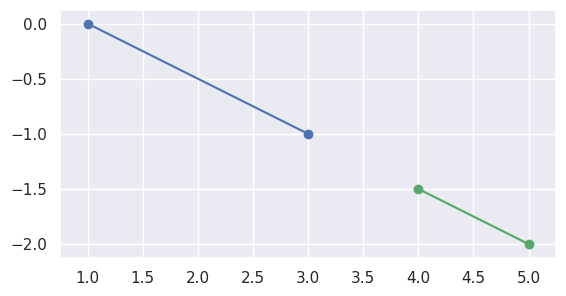
>>> start0 = np.asfortranarray([1.0, 0.0])
>>> delta0 = np.asfortranarray([2.0, -1.0])
>>> end0 = start0 + 1.0 * delta0
>>> start1 = start0 + 1.5 * delta0
>>> end1 = start0 + 2.0 * delta0
>>> disjoint, _ = parallel_lines_parameters(start0, end0, start1, end1)
>>> disjoint
True
but if the intervals overlap, like \(\left[0, 1\right]\) and \(\left[-1, \frac{1}{2}\right]\), the segments meet:
>>> start1 = start0 - 1.5 * delta0
>>> end1 = start0 + 0.5 * delta0
>>> disjoint, parameters = parallel_lines_parameters(
...     start0, end0, start1, end1)
>>> disjoint
False
>>> parameters
array([[0.  , 0.5 ],
       [0.75, 1.  ]])
Similarly, if the second interval completely contains the first, the segments meet:
>>> start1 = start0 + 4.5 * delta0
>>> end1 = start0 - 3.5 * delta0
>>> disjoint, parameters = parallel_lines_parameters(
...     start0, end0, start1, end1)
>>> disjoint
False
>>> parameters
array([[1.    , 0.    ],
       [0.4375, 0.5625]])
Note
This function doesn’t currently allow wiggle room around the desired value, i.e. the two values must be bitwise identical. However, the most “correct” version of this function likely should allow for some round off.
Note
There is also a Fortran implementation of this function, which will be used if it can be built.
- Parameters
start0 (numpy.ndarray) – A 1D NumPy
2-array that is the start vector \(S_0\) of the parametric line \(L_0(s)\).end0 (numpy.ndarray) – A 1D NumPy
2-array that is the end vector \(E_0\) of the parametric line \(L_0(s)\).start1 (numpy.ndarray) – A 1D NumPy
2-array that is the start vector \(S_1\) of the parametric line \(L_1(s)\).end1 (numpy.ndarray) – A 1D NumPy
2-array that is the end vector \(E_1\) of the parametric line \(L_1(s)\).
- Returns
A pair of
Flag indicating if the lines are disjoint.
An optional
2 x 2matrix ofs-tparameters only present if the lines aren’t disjoint. The first column will contain the parameters at the beginning of the shared segment and the second column will correspond to the end of the shared segment.
- Return type
Tuple[bool,Optional[numpy.ndarray] ]
-
bezier._py_curve_helpers.get_curvature(nodes, tangent_vec, s)¶ Compute the signed curvature of a curve at \(s\).
Computed via
\[\frac{B'(s) \times B''(s)}{\left\lVert B'(s) \right\rVert_2^3}\]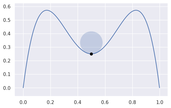
>>> nodes = np.asfortranarray([
...     [1.0, 0.75,  0.5, 0.25, 0.0],
...     [0.0, 2.0 , -2.0, 2.0 , 0.0],
... ])
>>> s = 0.5
>>> tangent_vec = evaluate_hodograph(s, nodes)
>>> tangent_vec
array([[-1.],
       [ 0.]])
>>> curvature = get_curvature(nodes, tangent_vec, s)
>>> curvature
-12.0
Note
There is also a Fortran implementation of this function, which will be used if it can be built.
- Parameters
nodes (numpy.ndarray) – The nodes of a curve.
tangent_vec (numpy.ndarray) – The already computed value of \(B'(s)\)
s (float) – The parameter value along the curve.
- Returns
The signed curvature.
- Return type
-
bezier._py_curve_helpers.newton_refine(nodes, point, s)¶ Refine a solution to \(B(s) = p\) using Newton’s method.
Computes updates via
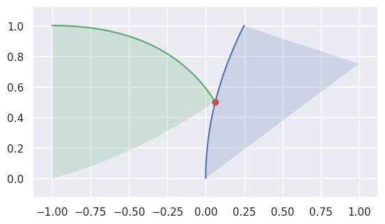
\[\mathbf{0} \approx \left(B\left(s_{\ast}\right) - p\right) + B'\left(s_{\ast}\right) \Delta s\]For example, consider the curve
\[\begin{split}B(s) = \left[\begin{array}{c} 0 \\ 0 \end{array}\right] (1 - s)^2 + \left[\begin{array}{c} 1 \\ 2 \end{array}\right] 2 (1 - s) s + \left[\begin{array}{c} 3 \\ 1 \end{array}\right] s^2\end{split}\]and the point \(B\left(\frac{1}{4}\right) = \frac{1}{16} \left[\begin{array}{c} 9 \\ 13 \end{array}\right]\).
Starting from the wrong point \(s = \frac{3}{4}\), we have
\[\begin{split}\begin{align*} p - B\left(\frac{1}{2}\right) &= -\frac{1}{2} \left[\begin{array}{c} 3 \\ 1 \end{array}\right] \\ B'\left(\frac{1}{2}\right) &= \frac{1}{2} \left[\begin{array}{c} 7 \\ -1 \end{array}\right] \\ \Longrightarrow \frac{1}{4} \left[\begin{array}{c c} 7 & -1 \end{array}\right] \left[\begin{array}{c} 7 \\ -1 \end{array}\right] \Delta s &= -\frac{1}{4} \left[\begin{array}{c c} 7 & -1 \end{array}\right] \left[\begin{array}{c} 3 \\ 1 \end{array}\right] \\ \Longrightarrow \Delta s &= -\frac{2}{5} \end{align*}\end{split}\]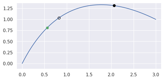
>>> nodes = np.asfortranarray([
...     [0.0, 1.0, 3.0],
...     [0.0, 2.0, 1.0],
... ])
>>> curve = bezier.Curve(nodes, degree=2)
>>> point = curve.evaluate(0.25)
>>> point
array([[0.5625],
       [0.8125]])
>>> s = 0.75
>>> new_s = newton_refine(nodes, point, s)
>>> 5 * (new_s - s)
-2.0
On curves that are not “valid” (i.e. \(B(s)\) is not injective with non-zero gradient), Newton’s method may break down and converge linearly:
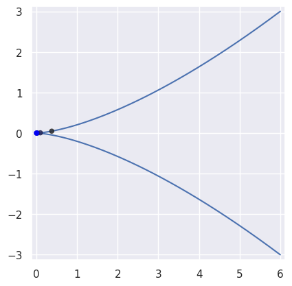
>>> nodes = np.asfortranarray([
...     [ 6.0, -2.0, -2.0, 6.0],
...     [-3.0,  3.0, -3.0, 3.0],
... ])
>>> curve = bezier.Curve(nodes, degree=3)
>>> expected = 0.5
>>> point = curve.evaluate(expected)
>>> point
array([[0.],
       [0.]])
>>> s_vals = [0.625, None, None, None, None, None]
>>> np.log2(abs(expected - s_vals[0]))
-3.0
>>> s_vals[1] = newton_refine(nodes, point, s_vals[0])
>>> np.log2(abs(expected - s_vals[1]))
-3.983...
>>> s_vals[2] = newton_refine(nodes, point, s_vals[1])
>>> np.log2(abs(expected - s_vals[2]))
-4.979...
>>> s_vals[3] = newton_refine(nodes, point, s_vals[2])
>>> np.log2(abs(expected - s_vals[3]))
-5.978...
>>> s_vals[4] = newton_refine(nodes, point, s_vals[3])
>>> np.log2(abs(expected - s_vals[4]))
-6.978...
>>> s_vals[5] = newton_refine(nodes, point, s_vals[4])
>>> np.log2(abs(expected - s_vals[5]))
-7.978...
Due to round-off, the Newton process terminates with an error that is not close to machine precision \(\varepsilon\) when \(\Delta s = 0\).
>>> s_vals = [0.625]
>>> new_s = newton_refine(nodes, point, s_vals[-1])
>>> while new_s not in s_vals:
...     s_vals.append(new_s)
...     new_s = newton_refine(nodes, point, s_vals[-1])
...
>>> terminal_s = s_vals[-1]
>>> terminal_s == newton_refine(nodes, point, terminal_s)
True
>>> 2.0**(-31) <= abs(terminal_s - 0.5) <= 2.0**(-28)
True
Due to round-off near the cusp, the final error resembles \(\sqrt{\varepsilon}\) rather than machine precision as expected.
Note
There is also a Fortran implementation of this function, which will be used if it can be built.
- Parameters
nodes (numpy.ndarray) – The nodes defining a Bézier curve.
point (numpy.ndarray) – A point on the curve.
s (float) – An “almost” solution to \(B(s) = p\).
- Returns
The updated value \(s + \Delta s\).
- Return type
-
bezier._py_triangle_helpers.classify_intersection(intersection, edge_nodes1, edge_nodes2)¶ Determine which curve is on the “inside of the intersection”.
Note
This is a helper used only by
Triangle.intersect().This is intended to be a helper for forming a
CurvedPolygonfrom the edge intersections of twoTriangle-s. In order to move from one intersection to another (or to the end of an edge), the interior edge must be determined at the point of intersection.The “typical” case is on the interior of both edges:
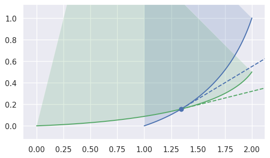
>>> nodes1 = np.asfortranarray([
...     [1.0, 1.75, 2.0],
...     [0.0, 0.25, 1.0],
... ])
>>> curve1 = bezier.Curve(nodes1, degree=2)
>>> nodes2 = np.asfortranarray([
...     [0.0, 1.6875, 2.0],
...     [0.0, 0.0625, 0.5],
... ])
>>> curve2 = bezier.Curve(nodes2, degree=2)
>>> s, t = 0.25, 0.5
>>> curve1.evaluate(s) == curve2.evaluate(t)
array([[ True],
       [ True]])
>>> tangent1 = hodograph(curve1, s)
>>> tangent1
array([[1.25],
       [0.75]])
>>> tangent2 = hodograph(curve2, t)
>>> tangent2
array([[2. ],
       [0.5]])
>>> intersection = Intersection(0, s, 0, t)
>>> edge_nodes1 = (nodes1, None, None)
>>> edge_nodes2 = (nodes2, None, None)
>>> classify_intersection(intersection, edge_nodes1, edge_nodes2)
<IntersectionClassification.FIRST: 0>
We determine the interior (i.e. left) one by using the right-hand rule: by embedding the tangent vectors in \(\mathbf{R}^3\), we compute
\[\begin{split}\left[\begin{array}{c} x_1'(s) \\ y_1'(s) \\ 0 \end{array}\right] \times \left[\begin{array}{c} x_2'(t) \\ y_2'(t) \\ 0 \end{array}\right] = \left[\begin{array}{c} 0 \\ 0 \\ x_1'(s) y_2'(t) - x_2'(t) y_1'(s) \end{array}\right].\end{split}\]If the cross product quantity \(B_1'(s) \times B_2'(t) = x_1'(s) y_2'(t) - x_2'(t) y_1'(s)\) is positive, then the first curve is “outside” / “to the right”, i.e. the second curve is interior. If the cross product is negative, the first curve is interior.
When \(B_1'(s) \times B_2'(t) = 0\), the tangent vectors are parallel, i.e. the intersection is a point of tangency:
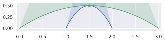
>>> nodes1 = np.asfortranarray([
...     [1.0, 1.5, 2.0],
...     [0.0, 1.0, 0.0],
... ])
>>> curve1 = bezier.Curve(nodes1, degree=2)
>>> nodes2 = np.asfortranarray([
...     [0.0, 1.5, 3.0],
...     [0.0, 1.0, 0.0],
... ])
>>> curve2 = bezier.Curve(nodes2, degree=2)
>>> s, t = 0.5, 0.5
>>> curve1.evaluate(s) == curve2.evaluate(t)
array([[ True],
       [ True]])
>>> intersection = Intersection(0, s, 0, t)
>>> edge_nodes1 = (nodes1, None, None)
>>> edge_nodes2 = (nodes2, None, None)
>>> classify_intersection(intersection, edge_nodes1, edge_nodes2)
<IntersectionClassification.TANGENT_SECOND: 4>
Depending on the direction of the parameterizations, the interior curve may change, but we can use the (signed) curvature of each curve at that point to determine which is on the interior:
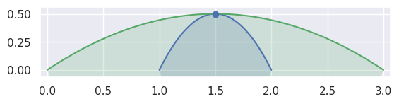
>>> nodes1 = np.asfortranarray([
...     [2.0, 1.5, 1.0],
...     [0.0, 1.0, 0.0],
... ])
>>> curve1 = bezier.Curve(nodes1, degree=2)
>>> nodes2 = np.asfortranarray([
...     [3.0, 1.5, 0.0],
...     [0.0, 1.0, 0.0],
... ])
>>> curve2 = bezier.Curve(nodes2, degree=2)
>>> s, t = 0.5, 0.5
>>> curve1.evaluate(s) == curve2.evaluate(t)
array([[ True],
       [ True]])
>>> intersection = Intersection(0, s, 0, t)
>>> edge_nodes1 = (nodes1, None, None)
>>> edge_nodes2 = (nodes2, None, None)
>>> classify_intersection(intersection, edge_nodes1, edge_nodes2)
<IntersectionClassification.TANGENT_FIRST: 3>
When the curves are moving in opposite directions at a point of tangency, there is no side to choose. Either the point of tangency is not part of any
CurvedPolygonintersection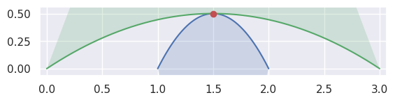
>>> nodes1 = np.asfortranarray([
...     [2.0, 1.5, 1.0],
...     [0.0, 1.0, 0.0],
... ])
>>> curve1 = bezier.Curve(nodes1, degree=2)
>>> nodes2 = np.asfortranarray([
...     [0.0, 1.5, 3.0],
...     [0.0, 1.0, 0.0],
... ])
>>> curve2 = bezier.Curve(nodes2, degree=2)
>>> s, t = 0.5, 0.5
>>> curve1.evaluate(s) == curve2.evaluate(t)
array([[ True],
       [ True]])
>>> intersection = Intersection(0, s, 0, t)
>>> edge_nodes1 = (nodes1, None, None)
>>> edge_nodes2 = (nodes2, None, None)
>>> classify_intersection(intersection, edge_nodes1, edge_nodes2)
<IntersectionClassification.OPPOSED: 2>
or the point of tangency is a “degenerate” part of two
CurvedPolygonintersections. It is “degenerate” because from one direction, the point should be classified asFIRSTand from another asSECOND.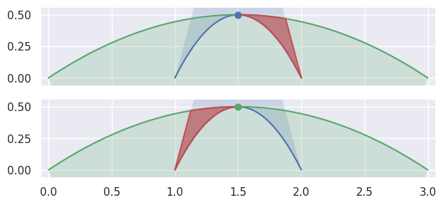
>>> nodes1 = np.asfortranarray([
...     [1.0, 1.5, 2.0],
...     [0.0, 1.0, 0.0],
... ])
>>> curve1 = bezier.Curve(nodes1, degree=2)
>>> nodes2 = np.asfortranarray([
...     [3.0, 1.5, 0.0],
...     [0.0, 1.0, 0.0],
... ])
>>> curve2 = bezier.Curve(nodes2, degree=2)
>>> s, t = 0.5, 0.5
>>> curve1.evaluate(s) == curve2.evaluate(t)
array([[ True],
       [ True]])
>>> intersection = Intersection(0, s, 0, t)
>>> edge_nodes1 = (nodes1, None, None)
>>> edge_nodes2 = (nodes2, None, None)
>>> classify_intersection(intersection, edge_nodes1, edge_nodes2)
<IntersectionClassification.TANGENT_BOTH: 6>
The
TANGENT_BOTHclassification can also occur if the curves are “kissing” but share a zero width interior at the point of tangency: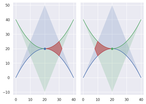
>>> nodes1 = np.asfortranarray([
...     [0.0, 20.0, 40.0],
...     [0.0, 40.0,  0.0],
... ])
>>> curve1 = bezier.Curve(nodes1, degree=2)
>>> nodes2 = np.asfortranarray([
...     [40.0, 20.0,  0.0],
...     [40.0,  0.0, 40.0],
... ])
>>> curve2 = bezier.Curve(nodes2, degree=2)
>>> s, t = 0.5, 0.5
>>> curve1.evaluate(s) == curve2.evaluate(t)
array([[ True],
       [ True]])
>>> intersection = Intersection(0, s, 0, t)
>>> edge_nodes1 = (nodes1, None, None)
>>> edge_nodes2 = (nodes2, None, None)
>>> classify_intersection(intersection, edge_nodes1, edge_nodes2)
<IntersectionClassification.TANGENT_BOTH: 6>
However, if the curvature of each curve is identical, we don’t try to distinguish further:
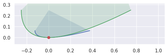
>>> nodes1 = np.asfortranarray([
...     [-0.125 , -0.125 , 0.375 ],
...     [ 0.0625, -0.0625, 0.0625],
... ])
>>> curve1 = bezier.Curve(nodes1, degree=2)
>>> nodes2 = np.asfortranarray([
...     [-0.25, -0.25, 0.75],
...     [ 0.25, -0.25, 0.25],
... ])
>>> curve2 = bezier.Curve(nodes2, degree=2)
>>> s, t = 0.5, 0.5
>>> curve1.evaluate(s) == curve2.evaluate(t)
array([[ True],
       [ True]])
>>> hodograph(curve1, s)
array([[0.5],
       [0. ]])
>>> hodograph(curve2, t)
array([[1.],
       [0.]])
>>> curvature(curve1, s)
2.0
>>> curvature(curve2, t)
2.0
>>> intersection = Intersection(0, s, 0, t)
>>> edge_nodes1 = (nodes1, None, None)
>>> edge_nodes2 = (nodes2, None, None)
>>> classify_intersection(intersection, edge_nodes1, edge_nodes2)
Traceback (most recent call last):
  ...
NotImplementedError: Tangent curves have same curvature.
In addition to points of tangency, intersections that happen at the end of an edge need special handling:
>>> nodes1a = np.asfortranarray([
...     [0.0, 4.5, 9.0 ],
...     [0.0, 0.0, 2.25],
... ])
>>> curve1a = bezier.Curve(nodes1a, degree=2)
>>> nodes2 = np.asfortranarray([
...     [11.25, 9.0, 2.75],
...     [ 0.0 , 4.5, 1.0 ],
... ])
>>> curve2 = bezier.Curve(nodes2, degree=2)
>>> s, t = 1.0, 0.375
>>> curve1a.evaluate(s) == curve2.evaluate(t)
array([[ True],
       [ True]])
>>> intersection = Intersection(0, s, 0, t)
>>> edge_nodes1 = (nodes1a, None, None)
>>> edge_nodes2 = (nodes2, None, None)
>>> classify_intersection(intersection, edge_nodes1, edge_nodes2)
Traceback (most recent call last):
  ...
ValueError: ('Intersection occurs at the end of an edge',
             's', 1.0, 't', 0.375)
>>>
>>> nodes1b = np.asfortranarray([
...     [9.0, 4.5, 0.0],
...     [2.25, 2.375, 2.5],
... ])
>>> curve1b = bezier.Curve(nodes1b, degree=2)
>>> curve1b.evaluate(0.0) == curve2.evaluate(t)
array([[ True],
       [ True]])
>>> intersection = Intersection(1, 0.0, 0, t)
>>> edge_nodes1 = (nodes1a, nodes1b, None)
>>> classify_intersection(intersection, edge_nodes1, edge_nodes2)
<IntersectionClassification.FIRST: 0>
As above, some intersections at the end of an edge are part of an actual intersection. However, some triangles may just “kiss” at a corner intersection:
>>> nodes1 = np.asfortranarray([
...     [0.25, 0.0, 0.0, 0.625, 0.5  , 1.0 ],
...     [1.0 , 0.5, 0.0, 0.875, 0.375, 0.75],
... ])
>>> triangle1 = bezier.Triangle(nodes1, degree=2)
>>> nodes2 = np.asfortranarray([
...     [0.0625, -0.25, -1.0, -0.5  , -1.0, -1.0],
...     [0.5   ,  1.0 ,  1.0,  0.125,  0.5,  0.0],
... ])
>>> triangle2 = bezier.Triangle(nodes2, degree=2)
>>> curve1, _, _ = triangle1.edges
>>> edge_nodes1 = [curve.nodes for curve in triangle1.edges]
>>> curve2, _, _ = triangle2.edges
>>> edge_nodes2 = [curve.nodes for curve in triangle2.edges]
>>> s, t = 0.5, 0.0
>>> curve1.evaluate(s) == curve2.evaluate(t)
array([[ True],
       [ True]])
>>> intersection = Intersection(0, s, 0, t)
>>> classify_intersection(intersection, edge_nodes1, edge_nodes2)
<IntersectionClassification.IGNORED_CORNER: 5>
Note
This assumes the intersection occurs in \(\mathbf{R}^2\) but doesn’t check this.
Note
This function doesn’t allow wiggle room / round-off when checking endpoints, nor when checking if the cross product is near zero, nor when curvatures are compared. However, the most “correct” version of this function likely should allow for some round off.
- Parameters
intersection (Intersection) – An intersection object.
edge_nodes1 (
Tuple[numpy.ndarray,numpy.ndarray,numpy.ndarray]) – The nodes of the three edges of the first triangle being intersected.edge_nodes2 (
Tuple[numpy.ndarray,numpy.ndarray,numpy.ndarray]) – The nodes of the three edges of the second triangle being intersected.
- Returns
The “inside” curve type, based on the classification enum.
- Return type
- Raises
ValueError – If the intersection occurs at the end of either curve involved. This is because we want to classify which curve to move forward on, and we can’t move past the end of a segment.
-
bezier._py_triangle_helpers.jacobian_det(nodes, degree, st_vals)¶ Compute \(\det(D B)\) at a set of values.
This requires that \(B \in \mathbf{R}^2\).
Note
This assumes but does not check that each
(s, t)inst_valsis inside the reference triangle.Warning
This relies on helpers in
bezierfor computing the Jacobian of the triangle. However, these helpers are not part of the public triangle and may change or be removed.>>> nodes = np.asfortranarray([ ... [0.0, 1.0, 2.0, 0.0, 1.5, 0.0], ... [0.0, 0.0, 0.0, 1.0, 1.5, 2.0], ... ]) >>> triangle = bezier.Triangle(nodes, degree=2) >>> st_vals = np.asfortranarray([ ... [0.25, 0.0 ], ... [0.75, 0.125], ... [0.5 , 0.5 ], ... ]) >>> s_vals, t_vals = st_vals.T >>> triangle.evaluate_cartesian_multi(st_vals) array([[0.5 , 1.59375, 1.25 ], [0. , 0.34375, 1.25 ]]) >>> # B(s, t) = [s(t + 2), t(s + 2)] >>> s_vals * (t_vals + 2) array([0.5 , 1.59375, 1.25 ]) >>> t_vals * (s_vals + 2) array([0. , 0.34375, 1.25 ]) >>> jacobian_det(nodes, 2, st_vals) array([4.5 , 5.75, 6. ]) >>> # det(DB) = 2(s + t + 2) >>> 2 * (s_vals + t_vals + 2) array([4.5 , 5.75, 6. ])
Note
There is also a Fortran implementation of this function, which will be used if it can be built.
- Parameters
nodes (numpy.ndarray) – Nodes defining a Bézier triangle \(B(s, t)\).
degree (int) – The degree of the triangle \(B\).
st_vals (numpy.ndarray) –
N x 2array of Cartesian inputs to Bézier triangles defined by \(B_s\) and \(B_t\).
- Returns
Array of all determinant values, one for each row in
st_vals.- Return type
-
bezier._py_triangle_intersection.newton_refine(nodes, degree, x_val, y_val, s, t)¶ Refine a solution to \(B(s, t) = p\) using Newton’s method.
Note
There is also a Fortran implementation of this function, which will be used if it can be built.
Computes updates via
\[\begin{split}\left[\begin{array}{c} 0 \\ 0 \end{array}\right] \approx \left(B\left(s_{\ast}, t_{\ast}\right) - \left[\begin{array}{c} x \\ y \end{array}\right]\right) + \left[\begin{array}{c c} B_s\left(s_{\ast}, t_{\ast}\right) & B_t\left(s_{\ast}, t_{\ast}\right) \end{array}\right] \left[\begin{array}{c} \Delta s \\ \Delta t \end{array}\right]\end{split}\]For example, (with weights \(\lambda_1 = 1 - s - t, \lambda_2 = s, \lambda_3 = t\)) consider the triangle
\[\begin{split}B(s, t) = \left[\begin{array}{c} 0 \\ 0 \end{array}\right] \lambda_1^2 + \left[\begin{array}{c} 1 \\ 0 \end{array}\right] 2 \lambda_1 \lambda_2 + \left[\begin{array}{c} 2 \\ 0 \end{array}\right] \lambda_2^2 + \left[\begin{array}{c} 2 \\ 1 \end{array}\right] 2 \lambda_1 \lambda_3 + \left[\begin{array}{c} 2 \\ 2 \end{array}\right] 2 \lambda_2 \lambda_1 + \left[\begin{array}{c} 0 \\ 2 \end{array}\right] \lambda_3^2\end{split}\]and the point \(B\left(\frac{1}{4}, \frac{1}{2}\right) = \frac{1}{4} \left[\begin{array}{c} 5 \\ 5 \end{array}\right]\).
Starting from the wrong point \(s = \frac{1}{2}, t = \frac{1}{4}\), we have
\[\begin{split}\begin{align*} \left[\begin{array}{c} x \\ y \end{array}\right] - B\left(\frac{1}{2}, \frac{1}{4}\right) &= \frac{1}{4} \left[\begin{array}{c} -1 \\ 2 \end{array}\right] \\ DB\left(\frac{1}{2}, \frac{1}{4}\right) &= \frac{1}{2} \left[\begin{array}{c c} 3 & 2 \\ 1 & 6 \end{array}\right] \\ \Longrightarrow \left[\begin{array}{c} \Delta s \\ \Delta t \end{array}\right] &= \frac{1}{32} \left[\begin{array}{c} -10 \\ 7 \end{array}\right] \end{align*}\end{split}\]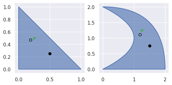
>>> nodes = np.asfortranarray([
...     [0.0, 1.0, 2.0, 2.0, 2.0, 0.0],
...     [0.0, 0.0, 0.0, 1.0, 2.0, 2.0],
... ])
>>> triangle = bezier.Triangle(nodes, degree=2)
>>> triangle.is_valid
True
>>> (x_val,), (y_val,) = triangle.evaluate_cartesian(0.25, 0.5)
>>> x_val, y_val
(1.25, 1.25)
>>> s, t = 0.5, 0.25
>>> new_s, new_t = newton_refine(nodes, 2, x_val, y_val, s, t)
>>> 32 * (new_s - s)
-10.0
>>> 32 * (new_t - t)
7.0
- Parameters
nodes (numpy.ndarray) – Array of nodes in a triangle.
degree (int) – The degree of the triangle.
x_val (float) – The \(x\)-coordinate of a point on the triangle.
y_val (float) – The \(y\)-coordinate of a point on the triangle.
s (float) – Approximate \(s\)-value to be refined.
t (float) – Approximate \(t\)-value to be refined.
- Returns
The refined \(s\) and \(t\) values.
- Return type
Types
-
class
bezier._py_intersection_helpers.IntersectionClassification¶ Enum classifying the “interior” curve in an intersection.
Provided as the output values for
classify_intersection().-
FIRST= 0¶ The first curve is on the interior.
-
SECOND= 1¶ The second curve is on the interior.
-
OPPOSED= 2¶ Tangent intersection with opposed interiors.
-
TANGENT_FIRST= 3¶ Tangent intersection, first curve is on the interior.
-
TANGENT_SECOND= 4¶ Tangent intersection, second curve is on the interior.
-
IGNORED_CORNER= 5¶ Intersection at a corner, interiors don’t intersect.
-
TANGENT_BOTH= 6¶ Tangent intersection, both curves are interior from some perspective.
-
COINCIDENT= 7¶ Intersection is actually an endpoint of a coincident segment.
-
COINCIDENT_UNUSED= 8¶ Unused because the edges are moving in opposite directions.
-
-
class
bezier._py_intersection_helpers.Intersection(index_first, s, index_second, t, interior_curve=None)¶ Representation of a curve-curve intersection.
- Parameters
index_first (int) – The index of the first curve within a list of curves. Expected to be used to index within the three edges of a triangle.
s (float) – The parameter along the first curve where the intersection occurs.
index_second (int) – The index of the second curve within a list of curves. Expected to be used to index within the three edges of a triangle.
t (float) – The parameter along the second curve where the intersection occurs.
interior_curve (
Optional[IntersectionClassification]) – The classification of the intersection.
-
interior_curve¶ Which of the curves is on the interior.
See
classify_intersection()for more details.
-
class
bezier._py_geometric_intersection.Linearization(curve, error)¶ A linearization of a curve.
This class is provided as a stand-in for a curve, so it provides a similar interface.
- Parameters
curve (SubdividedCurve) – A curve that is linearized.
error (float) – The linearization error. Expected to have been computed via
linearization_error().
-
curve¶ The curve that this linearization approximates.
- Type
-
start_node¶ The 1D start vector of this linearization.
- Type
-
end_node¶ The 1D end vector of this linearization.
- Type
-
subdivide()¶ Do-nothing method to match the
Curveinterface.- Returns
List of all subdivided parts, which is just the current object.
- Return type
Tuple[Linearization]
-
classmethod
from_shape(shape)¶ Try to linearize a curve (or an already linearized curve).
- Parameters
shape (
Union[SubdividedCurve,Linearization]) – A curve or an already linearized curve.- Returns
The (potentially linearized) curve.
- Return type
-
class
bezier._py_geometric_intersection.SubdividedCurve(nodes, original_nodes, start=0.0, end=1.0)¶ A data wrapper for a Bézier curve
To be used for intersection algorithm via repeated subdivision, where the
startandendparameters must be tracked.- Parameters
nodes (numpy.ndarray) – The control points of the current subdivided curve
original_nodes (numpy.ndarray) – The control points of the original curve used to define the current one (before subdivision began).
start (
Optional[float]) – The start parameter after subdivision.end (
Optional[float]) – The start parameter after subdivision.
-
subdivide()¶ Split the curve into a left and right half.
See
Curve.subdivide()for more information.- Returns
The left and right sub-curves.
- Return type