Algorithm Helpers
In an attempt to thoroughly vet each algorithm used in this library, each computation is split into small units that can be tested independently.
Though many of these computational units aren’t provided as part of the public interface of this library, they are still interesting. (Possibly) more importantly, it’s useful to see these algorithms at work.
In this document, these helper functions and objects are documented. This is to help with the exposition of the computation and does not imply that these are part of the stable public interface.
-
bezier._intersection_helpers._linearization_error(nodes)¶ Compute the maximum error of a linear approximation.
Helper for
Linearization, which is used during the curve-curve intersection process.We use the line
\[L(s) = v_0 (1 - s) + v_n s\]and compute a bound on the maximum error
\[\max_{s \in \left[0, 1\right]} \|B(s) - L(s)\|_2.\]Rather than computing the actual maximum (a tight bound), we use an upper bound via the remainder from Lagrange interpolation in each component. This leaves us with \(\frac{s(s - 1)}{2!}\) times the second derivative in each component.
The second derivative curve is degree \(d = n - 2\) and is given by
\[B''(s) = n(n - 1) \sum_{j = 0}^{d} \binom{d}{j} s^j (1 - s)^{d - j} \cdot \Delta^2 v_j\]Due to this form (and the convex combination property of Bézier Curves) we know each component of the second derivative will be bounded by the maximum of that component among the \(\Delta^2 v_j\).
For example, the curve
\[\begin{split}B(s) = \left[\begin{array}{c} 0 \\ 0 \end{array}\right] (1 - s)^2 + \left[\begin{array}{c} 3 \\ 1 \end{array}\right] 2s(1 - s) + \left[\begin{array}{c} 9 \\ -2 \end{array}\right] s^2\end{split}\]has \(B''(s) \equiv \left[\begin{array}{c} 6 \\ -8 \end{array}\right]\) which has norm \(10\) everywhere, hence the maximum error is
\[\left.\frac{s(1 - s)}{2!} \cdot 10\right|_{s = \frac{1}{2}} = \frac{5}{4}.\]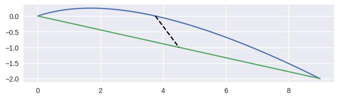
>>> nodes = np.asfortranarray([
...     [0.0,  0.0],
...     [3.0,  1.0],
...     [9.0, -2.0],
... ])
>>> linearization_error(nodes)
1.25
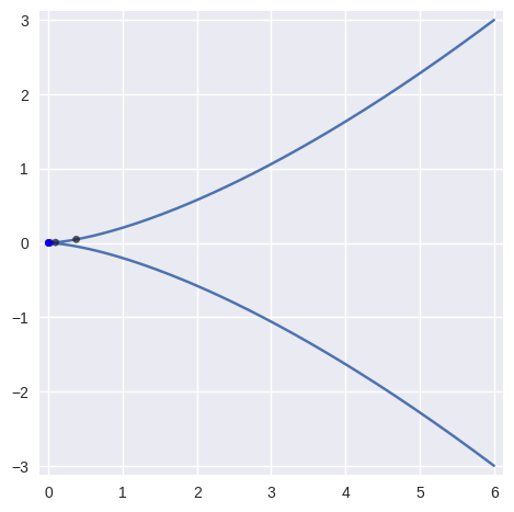
As a non-example, consider a “pathological” set of control points:
\[\begin{split}B(s) = \left[\begin{array}{c} 0 \\ 0 \end{array}\right] (1 - s)^3 + \left[\begin{array}{c} 5 \\ 12 \end{array}\right] 3s(1 - s)^2 + \left[\begin{array}{c} 10 \\ 24 \end{array}\right] 3s^2(1 - s) + \left[\begin{array}{c} 30 \\ 72 \end{array}\right] s^3\end{split}\]By construction, this lies on the line \(y = \frac{12x}{5}\), but the parametrization is cubic: \(12 \cdot x(s) = 5 \cdot y(s) = 180s(s^2 + 1)\). Hence, the fact that the curve is a line is not accounted for and we take the worse case among the nodes in:
\[\begin{split}B''(s) = 3 \cdot 2 \cdot \left( \left[\begin{array}{c} 0 \\ 0 \end{array}\right] (1 - s) + \left[\begin{array}{c} 15 \\ 36 \end{array}\right] s\right)\end{split}\]which gives a nonzero maximum error:
>>> nodes = np.asfortranarray([
...     [ 0.0,  0.0],
...     [ 5.0, 12.0],
...     [10.0, 24.0],
...     [30.0, 72.0],
... ])
>>> linearization_error(nodes)
29.25
Though it may seem that
0is a more appropriate answer, consider the goal of this function. We seek to linearize curves and then intersect the linear approximations. Then the \(s\)-values from the line-line intersection is lifted back to the curves. Thus the error \(\|B(s) - L(s)\|_2\) is more relevant than the underyling algebraic curve containing \(B(s)\).Note
It may be more appropriate to use a relative linearization error rather than the absolute error provided here. It’s unclear if the domain \(\left[0, 1\right]\) means the error is already adequately scaled or if the error should be scaled by the arc length of the curve or the (easier-to-compute) length of the line.
Note
There is also a Fortran implementation of this function, which will be used if it can be built.
Parameters: nodes (numpy.ndarray) – Nodes of a curve. Returns: The maximum error between the curve and the linear approximation. Return type: float
-
bezier._intersection_helpers._newton_refine(s, nodes1, t, nodes2)¶ Apply one step of 2D Newton’s method.
We want to use Newton’s method on the function
\[F(s, t) = B_1(s) - B_2(t)\]to refine \(\left(s_{\ast}, t_{\ast}\right)\). Using this, and the Jacobian \(DF\), we “solve”
\[\begin{split}\left[\begin{array}{c} 0 \\ 0 \end{array}\right] \approx F\left(s_{\ast} + \Delta s, t_{\ast} + \Delta t\right) \approx F\left(s_{\ast}, t_{\ast}\right) + \left[\begin{array}{c c} B_1'\left(s_{\ast}\right) & - B_2'\left(t_{\ast}\right) \end{array}\right] \left[\begin{array}{c} \Delta s \\ \Delta t \end{array}\right]\end{split}\]and refine with the component updates \(\Delta s\) and \(\Delta t\).
Note
This implementation assumes the curves live in \(\mathbf{R}^2\).
For example, the curves
\[\begin{split}\begin{align*} B_1(s) &= \left[\begin{array}{c} 0 \\ 0 \end{array}\right] (1 - s)^2 + \left[\begin{array}{c} 2 \\ 4 \end{array}\right] 2s(1 - s) + \left[\begin{array}{c} 4 \\ 0 \end{array}\right] s^2 \\ B_2(t) &= \left[\begin{array}{c} 2 \\ 0 \end{array}\right] (1 - t) + \left[\begin{array}{c} 0 \\ 3 \end{array}\right] t \end{align*}\end{split}\]intersect at the point \(B_1\left(\frac{1}{4}\right) = B_2\left(\frac{1}{2}\right) = \frac{1}{2} \left[\begin{array}{c} 2 \\ 3 \end{array}\right]\).
However, starting from the wrong point we have
\[\begin{split}\begin{align*} F\left(\frac{3}{8}, \frac{1}{4}\right) &= \frac{1}{8} \left[\begin{array}{c} 0 \\ 9 \end{array}\right] \\ DF\left(\frac{3}{8}, \frac{1}{4}\right) &= \left[\begin{array}{c c} 4 & 2 \\ 2 & -3 \end{array}\right] \\ \Longrightarrow \left[\begin{array}{c} \Delta s \\ \Delta t \end{array}\right] &= \frac{9}{64} \left[\begin{array}{c} -1 \\ 2 \end{array}\right]. \end{align*}\end{split}\]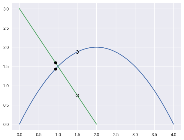
>>> nodes1 = np.asfortranarray([
...     [0.0, 0.0],
...     [2.0, 4.0],
...     [4.0, 0.0],
... ])
>>> nodes2 = np.asfortranarray([
...     [2.0, 0.0],
...     [0.0, 3.0],
... ])
>>> s, t = 0.375, 0.25
>>> new_s, new_t = newton_refine(s, nodes1, t, nodes2)
>>> 64.0 * (new_s - s)
-9.0
>>> 64.0 * (new_t - t)
18.0
For “typical” curves, we converge to a solution quadratically. This means that the number of correct digits doubles every iteration (until machine precision is reached).
>>> nodes1 = np.asfortranarray([
...     [0.0 ,  0.0],
...     [0.25,  2.0],
...     [0.5 , -2.0],
...     [0.75,  2.0],
...     [1.0 ,  0.0],
... ])
>>> nodes2 = np.asfortranarray([
...     [0.0 , 1.0],
...     [0.25, 0.5],
...     [0.5 , 0.5],
...     [0.75, 0.5],
...     [1.0 , 0.0],
... ])
>>> # The expected intersection is the only real root of
>>> # 28 s^3 - 30 s^2 + 9 s - 1.
>>> omega = (28.0 * np.sqrt(17.0) + 132.0)**(1.0 / 3.0) / 28.0
>>> expected = 5.0 / 14.0 + omega + 1 / (49.0 * omega)
>>> s_vals = [0.625, None, None, None, None]
>>> t = 0.625
>>> np.log2(abs(expected - s_vals[0]))
-4.399...
>>> s_vals[1], t = newton_refine(s_vals[0], nodes1, t, nodes2)
>>> np.log2(abs(expected - s_vals[1]))
-7.901...
>>> s_vals[2], t = newton_refine(s_vals[1], nodes1, t, nodes2)
>>> np.log2(abs(expected - s_vals[2]))
-16.010...
>>> s_vals[3], t = newton_refine(s_vals[2], nodes1, t, nodes2)
>>> np.log2(abs(expected - s_vals[3]))
-32.110...
>>> s_vals[4], t = newton_refine(s_vals[3], nodes1, t, nodes2)
>>> s_vals[4] == expected
True
However, when the intersection occurs at a point of tangency, the convergence becomes linear. This means that the number of correct digits added each iteration is roughly constant.
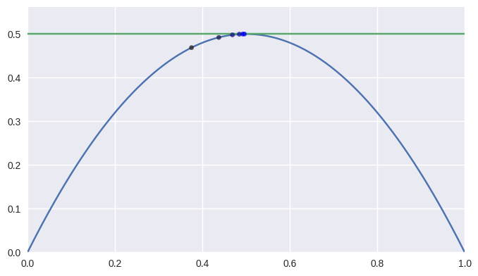
>>> nodes1 = np.asfortranarray([
...     [0.0, 0.0],
...     [0.5, 1.0],
...     [1.0, 0.0],
... ])
>>> nodes2 = np.asfortranarray([
...     [0.0, 0.5],
...     [1.0, 0.5],
... ])
>>> expected = 0.5
>>> s_vals = [0.375, None, None, None, None, None]
>>> t = 0.375
>>> np.log2(abs(expected - s_vals[0]))
-3.0
>>> s_vals[1], t = newton_refine(s_vals[0], nodes1, t, nodes2)
>>> np.log2(abs(expected - s_vals[1]))
-4.0
>>> s_vals[2], t = newton_refine(s_vals[1], nodes1, t, nodes2)
>>> np.log2(abs(expected - s_vals[2]))
-5.0
>>> s_vals[3], t = newton_refine(s_vals[2], nodes1, t, nodes2)
>>> np.log2(abs(expected - s_vals[3]))
-6.0
>>> s_vals[4], t = newton_refine(s_vals[3], nodes1, t, nodes2)
>>> np.log2(abs(expected - s_vals[4]))
-7.0
>>> s_vals[5], t = newton_refine(s_vals[4], nodes1, t, nodes2)
>>> np.log2(abs(expected - s_vals[5]))
-8.0
Unfortunately, the process terminates with an error that is not close to machine precision \(\varepsilon\) when \(\Delta s = \Delta t = 0\).
>>> s1 = t1 = 0.5 - 0.5**27
>>> np.log2(0.5 - s1)
-27.0
>>> s2, t2 = newton_refine(s1, nodes1, t1, nodes2)
>>> s2 == t2
True
>>> np.log2(0.5 - s2)
-28.0
>>> s3, t3 = newton_refine(s2, nodes1, t2, nodes2)
>>> s3 == t3 == s2
True
Due to round-off near the point of tangency, the final error resembles \(\sqrt{\varepsilon}\) rather than machine precision as expected.
Note
The following is not implemented in this function. It’s just an exploration on how the shortcomings might be addressed.
However, this can be overcome. At the point of tangency, we want \(B_1'(s) \parallel B_2'(t)\). This can be checked numerically via
\[B_1'(s) \times B_2'(t) = 0.\]For the last example (the one that converges linearly), this is
\[\begin{split}0 = \left[\begin{array}{c} 1 \\ 2 - 4s \end{array}\right] \times \left[\begin{array}{c} 1 \\ 0 \end{array}\right] = 4 s - 2.\end{split}\]With this, we can modify Newton’s method to find a zero of the over-determined system
\[\begin{split}G(s, t) = \left[\begin{array}{c} B_0(s) - B_1(t) \\ B_1'(s) \times B_2'(t) \end{array}\right] = \left[\begin{array}{c} s - t \\ 2 s (1 - s) - \frac{1}{2} \\ 4 s - 2\end{array}\right].\end{split}\]Since \(DG\) is \(3 \times 2\), we can’t invert it. However, we can find a least-squares solution:
\[\begin{split}\left(DG^T DG\right) \left[\begin{array}{c} \Delta s \\ \Delta t \end{array}\right] = -DG^T G.\end{split}\]This only works if \(DG\) has full rank. In this case, it does since the submatrix containing the first and last rows has rank two:
\[\begin{split}DG = \left[\begin{array}{c c} 1 & -1 \\ 2 - 4 s & 0 \\ 4 & 0 \end{array}\right].\end{split}\]Though this avoids a singular system, the normal equations have a condition number that is the square of the condition number of the matrix.
Starting from \(s = t = \frac{3}{8}\) as above:
>>> s0, t0 = 0.375, 0.375
>>> np.log2(0.5 - s0)
-3.0
>>> s1, t1 = modified_update(s0, t0)
>>> s1 == t1
True
>>> 1040.0 * s1
519.0
>>> np.log2(0.5 - s1)
-10.022...
>>> s2, t2 = modified_update(s1, t1)
>>> s2 == t2
True
>>> np.log2(0.5 - s2)
-31.067...
>>> s3, t3 = modified_update(s2, t2)
>>> s3 == t3 == 0.5
True
Parameters: - s (float) – Parameter of a near-intersection along the first curve.
- nodes1 (numpy.ndarray) – Nodes of first curve forming intersection.
- t (float) – Parameter of a near-intersection along the second curve.
- nodes2 (numpy.ndarray) – Nodes of second curve forming intersection.
Returns: The refined parameters from a single Newton step.
Return type:
-
bezier._intersection_helpers._segment_intersection(start0, end0, start1, end1)¶ Determine the intersection of two line segments.
Assumes each line is parametric
\[\begin{split}\begin{alignat*}{2} L_0(s) &= S_0 (1 - s) + E_0 s &&= S_0 + s \Delta_0 \\ L_1(t) &= S_1 (1 - t) + E_1 t &&= S_1 + t \Delta_1. \end{alignat*}\end{split}\]To solve \(S_0 + s \Delta_0 = S_1 + t \Delta_1\), we use the cross product:
\[\left(S_0 + s \Delta_0\right) \times \Delta_1 = \left(S_1 + t \Delta_1\right) \times \Delta_1 \Longrightarrow s \left(\Delta_0 \times \Delta_1\right) = \left(S_1 - S_0\right) \times \Delta_1.\]Similarly
\[\Delta_0 \times \left(S_0 + s \Delta_0\right) = \Delta_0 \times \left(S_1 + t \Delta_1\right) \Longrightarrow \left(S_1 - S_0\right) \times \Delta_0 = \Delta_0 \times \left(S_0 - S_1\right) = t \left(\Delta_0 \times \Delta_1\right).\]Note
Since our points are in \(\mathbf{R}^2\), the “traditional” cross product in \(\mathbf{R}^3\) will always point in the \(z\) direction, so in the above we mean the \(z\) component of the cross product, rather than the entire vector.
For example, the diagonal lines
\[\begin{split}\begin{align*} L_0(s) &= \left[\begin{array}{c} 0 \\ 0 \end{array}\right] (1 - s) + \left[\begin{array}{c} 2 \\ 2 \end{array}\right] s \\ L_1(t) &= \left[\begin{array}{c} -1 \\ 2 \end{array}\right] (1 - t) + \left[\begin{array}{c} 1 \\ 0 \end{array}\right] t \end{align*}\end{split}\]intersect at \(L_0\left(\frac{1}{4}\right) = L_1\left(\frac{3}{4}\right) = \frac{1}{2} \left[\begin{array}{c} 1 \\ 1 \end{array}\right]\).
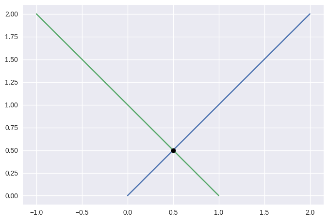
>>> start0 = np.asfortranarray([[0.0, 0.0]])
>>> end0 = np.asfortranarray([[2.0, 2.0]])
>>> start1 = np.asfortranarray([[-1.0, 2.0]])
>>> end1 = np.asfortranarray([[1.0, 0.0]])
>>> s, t, _ = segment_intersection(start0, end0, start1, end1)
>>> s
0.25
>>> t
0.75
Taking the parallel (but different) lines
\[\begin{split}\begin{align*} L_0(s) &= \left[\begin{array}{c} 1 \\ 0 \end{array}\right] (1 - s) + \left[\begin{array}{c} 0 \\ 1 \end{array}\right] s \\ L_1(t) &= \left[\begin{array}{c} -1 \\ 3 \end{array}\right] (1 - t) + \left[\begin{array}{c} 3 \\ -1 \end{array}\right] t \end{align*}\end{split}\]we should be able to determine that the lines don’t intersect, but this function is not meant for that check:
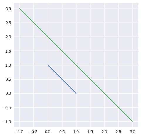
>>> start0 = np.asfortranarray([[1.0, 0.0]])
>>> end0 = np.asfortranarray([[0.0, 1.0]])
>>> start1 = np.asfortranarray([[-1.0, 3.0]])
>>> end1 = np.asfortranarray([[3.0, -1.0]])
>>> _, _, success = segment_intersection(start0, end0, start1, end1)
>>> bool(success)
False
Instead, we use
parallel_different():>>> bool(parallel_different(start0, end0, start1, end1)) True
Note
There is also a Fortran implementation of this function, which will be used if it can be built.
Parameters: - start0 (numpy.ndarray) – A 1x2 NumPy array that is the start vector \(S_0\) of the parametric line \(L_0(s)\).
- end0 (numpy.ndarray) – A 1x2 NumPy array that is the end vector \(E_0\) of the parametric line \(L_0(s)\).
- start1 (numpy.ndarray) – A 1x2 NumPy array that is the start vector \(S_1\) of the parametric line \(L_1(s)\).
- end1 (numpy.ndarray) – A 1x2 NumPy array that is the end vector \(E_1\) of the parametric line \(L_1(s)\).
Returns: Pair of \(s_{\ast}\) and \(t_{\ast}\) such that the lines intersect: \(L_0\left(s_{\ast}\right) = L_1\left(t_{\ast}\right)\) and then a boolean indicating if an intersection was found.
Return type:
-
bezier._intersection_helpers._parallel_different(start0, end0, start1, end1)¶ Checks if two parallel lines ever meet.
Meant as a back-up when
segment_intersection()fails.Note
This function assumes but never verifies that the lines are parallel.
In the case that the segments are parallel and lie on the exact same line, finding a unique intersection is not possible. However, if they are parallel but on different lines, then there is a guarantee of no intersection.
In
segment_intersection(), we utilized the normal form of the lines (via the cross product):\[\begin{split}\begin{align*} L_0(s) \times \Delta_0 &\equiv S_0 \times \Delta_0 \\ L_1(t) \times \Delta_1 &\equiv S_1 \times \Delta_1 \end{align*}\end{split}\]So, we can detect if \(S_1\) is on the first line by checking if
\[S_0 \times \Delta_0 \stackrel{?}{=} S_1 \times \Delta_0.\]If it is not on the first line, then we are done, the segments don’t meet:
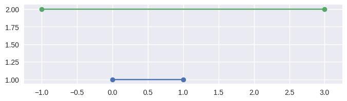
>>> # Line: y = 1
>>> start0 = np.asfortranarray([[0.0, 1.0]])
>>> end0 = np.asfortranarray([[1.0, 1.0]])
>>> # Vertical shift up: y = 2
>>> start1 = np.asfortranarray([[-1.0, 2.0]])
>>> end1 = np.asfortranarray([[3.0, 2.0]])
>>> bool(parallel_different(start0, end0, start1, end1))
True
If \(S_1\) is on the first line, we want to check that \(S_1\) and \(E_1\) define parameters outside of \(\left[0, 1\right]\). To compute these parameters:
\[L_1(t) = S_0 + s_{\ast} \Delta_0 \Longrightarrow s_{\ast} = \frac{\Delta_0^T \left( L_1(t) - S_0\right)}{\Delta_0^T \Delta_0}.\]For example, the intervals \(\left[0, 1\right]\) and \(\left[\frac{3}{2}, 2\right]\) (via \(S_1 = S_0 + \frac{3}{2} \Delta_0\) and \(E_1 = S_0 + 2 \Delta_0\)) correspond to segments that don’t meet:
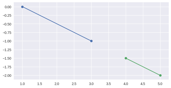
>>> start0 = np.asfortranarray([[1.0, 0.0]])
>>> delta0 = np.asfortranarray([[2.0, -1.0]])
>>> end0 = start0 + 1.0 * delta0
>>> start1 = start0 + 1.5 * delta0
>>> end1 = start0 + 2.0 * delta0
>>> bool(parallel_different(start0, end0, start1, end1))
True
but if the intervals overlap, like \(\left[0, 1\right]\) and \(\left[-1, \frac{1}{2}\right]\), the segments meet:
>>> start1 = start0 - 1.0 * delta0
>>> end1 = start0 + 0.5 * delta0
>>> bool(parallel_different(start0, end0, start1, end1))
False
Similarly, if the second interval completely contains the first, the segments meet:
>>> start1 = start0 + 3.0 * delta0
>>> end1 = start0 - 2.0 * delta0
>>> bool(parallel_different(start0, end0, start1, end1))
False
Note
This function doesn’t currently allow wiggle room around the desired value, i.e. the two values must be bitwise identical. However, the most “correct” version of this function likely should allow for some round off.
Parameters: - start0 (numpy.ndarray) – A 1x2 NumPy array that is the start vector \(S_0\) of the parametric line \(L_0(s)\).
- end0 (numpy.ndarray) – A 1x2 NumPy array that is the end vector \(E_0\) of the parametric line \(L_0(s)\).
- start1 (numpy.ndarray) – A 1x2 NumPy array that is the start vector \(S_1\) of the parametric line \(L_1(s)\).
- end1 (numpy.ndarray) – A 1x2 NumPy array that is the end vector \(E_1\) of the parametric line \(L_1(s)\).
Returns: Indicating if the lines are different.
Return type:
-
bezier._curve_helpers.get_curvature(nodes, degree, tangent_vec, s)¶ Compute the signed curvature of a curve at \(s\).
Computed via
\[\frac{B'(s) \times B''(s)}{\left\lVert B'(s) \right\rVert_2^3}\]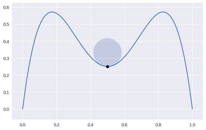
>>> nodes = np.asfortranarray([
...     [1.0 ,  0.0],
...     [0.75,  2.0],
...     [0.5 , -2.0],
...     [0.25,  2.0],
...     [0.0 ,  0.0],
... ])
>>> s = 0.5
>>> tangent_vec = hodograph(nodes, s)
>>> tangent_vec
array([[-1., 0.]])
>>> curvature = get_curvature(nodes, 4, tangent_vec, s)
>>> curvature
-12.0
Parameters: - nodes (numpy.ndarray) – The nodes of a curve.
- degree (int) – The degree of the curve.
- tangent_vec (numpy.ndarray) – The already computed value of \(B'(s)\)
- s (float) – The parameter value along the curve.
Returns: The signed curvature.
Return type:
-
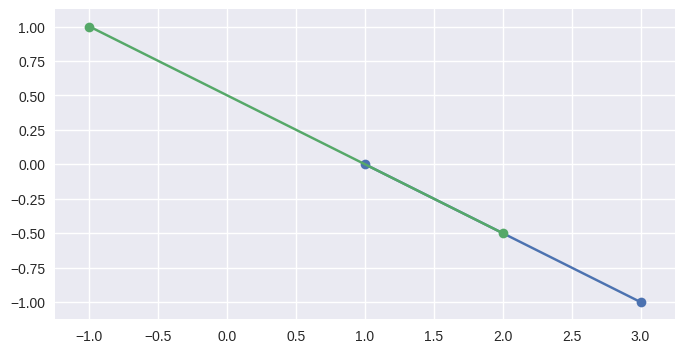
bezier._curve_helpers.newton_refine(nodes, degree, point, s)¶ Refine a solution to \(B(s) = p\) using Newton’s method.
Computes updates via
\[\mathbf{0} \approx \left(B\left(s_{\ast}\right) - p\right) + B'\left(s_{\ast}\right) \Delta s\]For example, consider the curve
\[\begin{split}B(s) = \left[\begin{array}{c} 0 \\ 0 \end{array}\right] (1 - s)^2 + \left[\begin{array}{c} 1 \\ 2 \end{array}\right] 2 (1 - s) s + \left[\begin{array}{c} 3 \\ 1 \end{array}\right] s^2\end{split}\]and the point \(B\left(\frac{1}{4}\right) = \frac{1}{16} \left[\begin{array}{c} 9 \\ 13 \end{array}\right]\).
Starting from the wrong point \(s = \frac{3}{4}\), we have
\[\begin{split}\begin{align*} p - B\left(\frac{1}{2}\right) &= -\frac{1}{2} \left[\begin{array}{c} 3 \\ 1 \end{array}\right] \\ B'\left(\frac{1}{2}\right) &= \frac{1}{2} \left[\begin{array}{c} 7 \\ -1 \end{array}\right] \\ \Longrightarrow \frac{1}{4} \left[\begin{array}{c c} 7 & -1 \end{array}\right] \left[\begin{array}{c} 7 \\ -1 \end{array}\right] \Delta s &= -\frac{1}{4} \left[\begin{array}{c c} 7 & -1 \end{array}\right] \left[\begin{array}{c} 3 \\ 1 \end{array}\right] \\ \Longrightarrow \Delta s &= -\frac{2}{5} \end{align*}\end{split}\]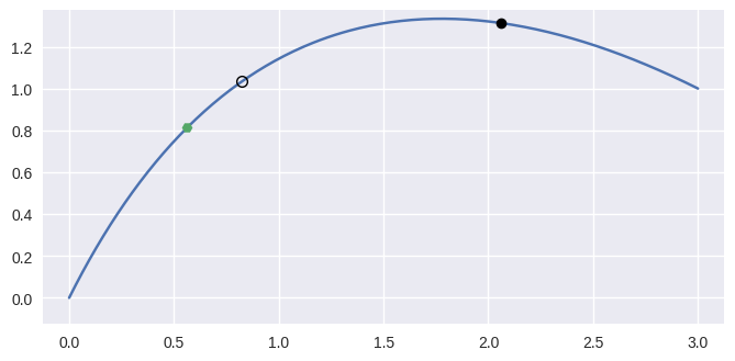
>>> nodes = np.asfortranarray([
...     [0.0, 0.0],
...     [1.0, 2.0],
...     [3.0, 1.0],
... ])
>>> curve = bezier.Curve(nodes, degree=2)
>>> point = curve.evaluate(0.25)
>>> point
array([[ 0.5625, 0.8125]])
>>> s = 0.75
>>> new_s = newton_refine(nodes, 2, point, s)
>>> 5 * (new_s - s)
-2.0
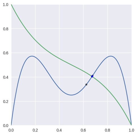
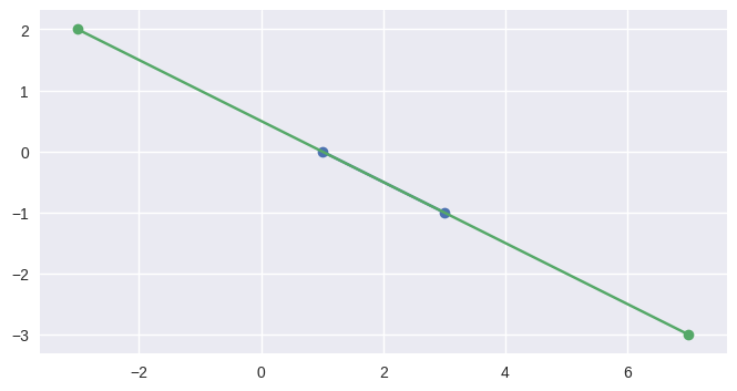
On curves that are not “valid” (i.e. \(B(s)\) is not injective with non-zero gradient), Newton’s method may break down and converge linearly:
>>> nodes = np.asfortranarray([
...     [ 6.0, -3.0],
...     [-2.0,  3.0],
...     [-2.0, -3.0],
...     [ 6.0,  3.0],
... ])
>>> curve = bezier.Curve(nodes, degree=3)
>>> expected = 0.5
>>> point = curve.evaluate(expected)
>>> point
array([[ 0., 0.]])
>>> s_vals = [0.625, None, None, None, None, None]
>>> np.log2(abs(expected - s_vals[0]))
-3.0
>>> s_vals[1] = newton_refine(nodes, 3, point, s_vals[0])
>>> np.log2(abs(expected - s_vals[1]))
-3.983...
>>> s_vals[2] = newton_refine(nodes, 3, point, s_vals[1])
>>> np.log2(abs(expected - s_vals[2]))
-4.979...
>>> s_vals[3] = newton_refine(nodes, 3, point, s_vals[2])
>>> np.log2(abs(expected - s_vals[3]))
-5.978...
>>> s_vals[4] = newton_refine(nodes, 3, point, s_vals[3])
>>> np.log2(abs(expected - s_vals[4]))
-6.978...
>>> s_vals[5] = newton_refine(nodes, 3, point, s_vals[4])
>>> np.log2(abs(expected - s_vals[5]))
-7.978...
Due to round-off, the Newton process terminates with an error that is not close to machine precision \(\varepsilon\) when \(\Delta s = 0\).
>>> s_vals = [0.625]
>>> new_s = newton_refine(nodes, 3, point, s_vals[-1])
>>> while new_s not in s_vals:
...     s_vals.append(new_s)
...     new_s = newton_refine(nodes, 3, point, s_vals[-1])
...
>>> terminal_s = s_vals[-1]
>>> terminal_s == newton_refine(nodes, 3, point, terminal_s)
True
>>> 2.0**(-31) <= abs(terminal_s - 0.5) <= 2.0**(-29)
True
Due to round-off near the cusp, the final error resembles \(\sqrt{\varepsilon}\) rather than machine precision as expected.
Parameters: - nodes (numpy.ndarray) – The nodes defining a Bézier curve.
- degree (int) – The degree of the curve (assumed to be one less than
the number of
nodes. - point (numpy.ndarray) – A point on the curve.
- s (float) – An “almost” solution to \(B(s) = p\).
Returns: The updated value \(s + \Delta s\).
Return type:
-
class
bezier._intersection_helpers.Intersection(first, s, second, t, point=None, interior_curve=None)¶ Representation of a curve-curve intersection.
Parameters: - first (Curve) – The “first” curve in the intersection.
- s (float) – The parameter along
firstwhere the intersection occurs. - second (Curve) – The “second” curve in the intersection.
- t (float) – The parameter along
secondwhere the intersection occurs. - point (
Optional[numpy.ndarray]) – The point where the two curves actually intersect. - interior_curve (
Optional[IntersectionClassification]) – The classification of the intersection.
-
get_point()¶ The point where the intersection occurs.
This exists primarily for
Curve.intersect().Returns: The point where the intersection occurs. Returns pointif stored on the current value, otherwise computes the value on the fly.Return type: numpy.ndarray
-
class
bezier._intersection_helpers.Linearization(curve, error)¶ A linearization of a curve.
This class is provided as a stand-in for a curve, so it provides a similar interface.
Parameters: -
classmethod
from_shape(shape)¶ Try to linearize a curve (or an already linearized curve).
Parameters: shape ( Union[Curve,Linearization]) – A curve or an already linearized curve.Returns: The (potentially linearized) curve. Return type: Union[Curve,Linearization]
-
subdivide()¶ Do-nothing method to match the
Curveinterface.Returns: List of all subdivided parts, which is just the current object. Return type: Tuple[Linearization]
-
classmethod
-
class
bezier._surface_helpers.IntersectionClassification¶ Enum classifying the “interior” curve in an intersection.
Provided as the output values for
classify_intersection().
-
bezier._surface_helpers.newton_refine(nodes, degree, x_val, y_val, s, t)¶ Refine a solution to \(B(s, t) = p\) using Newton’s method.
Computes updates via
\[\begin{split}\left[\begin{array}{c} 0 \\ 0 \end{array}\right] \approx \left(B\left(s_{\ast}, t_{\ast}\right) - \left[\begin{array}{c} x \\ y \end{array}\right]\right) + \left[\begin{array}{c c} B_s\left(s_{\ast}, t_{\ast}\right) & B_t\left(s_{\ast}, t_{\ast}\right) \end{array}\right] \left[\begin{array}{c} \Delta s \\ \Delta t \end{array}\right]\end{split}\]For example, (with weights \(\lambda_1 = 1 - s - t, \lambda_2 = s, \lambda_3 = t\)) consider the surface
\[\begin{split}B(s, t) = \left[\begin{array}{c} 0 \\ 0 \end{array}\right] \lambda_1^2 + \left[\begin{array}{c} 1 \\ 0 \end{array}\right] 2 \lambda_1 \lambda_2 + \left[\begin{array}{c} 2 \\ 0 \end{array}\right] \lambda_2^2 + \left[\begin{array}{c} 2 \\ 1 \end{array}\right] 2 \lambda_1 \lambda_3 + \left[\begin{array}{c} 2 \\ 2 \end{array}\right] 2 \lambda_2 \lambda_1 + \left[\begin{array}{c} 0 \\ 2 \end{array}\right] \lambda_3^2\end{split}\]and the point \(B\left(\frac{1}{4}, \frac{1}{2}\right) = \frac{1}{4} \left[\begin{array}{c} 5 \\ 5 \end{array}\right]\).
Starting from the wrong point \(s = \frac{1}{2}, t = \frac{1}{4}\), we have
\[\begin{split}\begin{align*} \left[\begin{array}{c} x \\ y \end{array}\right] - B\left(\frac{1}{2}, \frac{1}{4}\right) &= \frac{1}{4} \left[\begin{array}{c} -1 \\ 2 \end{array}\right] \\ DB\left(\frac{1}{2}, \frac{1}{4}\right) &= \frac{1}{2} \left[\begin{array}{c c} 3 & 2 \\ 1 & 6 \end{array}\right] \\ \Longrightarrow \left[\begin{array}{c} \Delta s \\ \Delta t \end{array}\right] &= \frac{1}{32} \left[\begin{array}{c} -10 \\ 7 \end{array}\right] \end{align*}\end{split}\]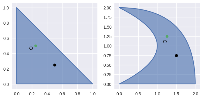
>>> nodes = np.asfortranarray([
...     [0.0, 0.0],
...     [1.0, 0.0],
...     [2.0, 0.0],
...     [2.0, 1.0],
...     [2.0, 2.0],
...     [0.0, 2.0],
... ])
>>> surface = bezier.Surface(nodes, degree=2)
>>> surface.is_valid
True
>>> (x_val, y_val), = surface.evaluate_cartesian(0.25, 0.5)
>>> x_val, y_val
(1.25, 1.25)
>>> s, t = 0.5, 0.25
>>> new_s, new_t = newton_refine(nodes, 2, x_val, y_val, s, t)
>>> 32 * (new_s - s)
-10.0
>>> 32 * (new_t - t)
7.0
Parameters: - nodes (numpy.ndarray) – Array of nodes in a surface.
- degree (int) – The degree of the surface.
- x_val (float) – The \(x\)-coordinate of a point on the surface.
- y_val (float) – The \(y\)-coordinate of a point on the surface.
- s (float) – Approximate \(s\)-value to be refined.
- t (float) – Approximate \(t\)-value to be refined.
Returns: The refined \(s\) and \(t\) values.
Return type:
-
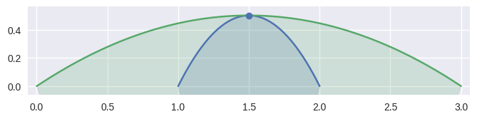
bezier._surface_helpers.classify_intersection(intersection)¶ Determine which curve is on the “inside of the intersection”.
This is intended to be a helper for forming a
CurvedPolygonfrom the edge intersections of twoSurface-s. In order to move from one intersection to another (or to the end of an edge), the interior edge must be determined at the point of intersection.The “typical” case is on the interior of both edges:
>>> nodes1 = np.asfortranarray([
...     [1.0 , 0.0 ],
...     [1.75, 0.25],
...     [2.0 , 1.0 ],
... ])
>>> curve1 = bezier.Curve(nodes1, degree=2)
>>> nodes2 = np.asfortranarray([
...     [0.0   , 0.0   ],
...     [1.6875, 0.0625],
...     [2.0   , 0.5   ],
... ])
>>> curve2 = bezier.Curve(nodes2, degree=2)
>>> s, t = 0.25, 0.5
>>> curve1.evaluate(s) == curve2.evaluate(t)
array([[ True, True]], dtype=bool)
>>> tangent1 = hodograph(curve1, s)
>>> tangent1
array([[ 1.25, 0.75]])
>>> tangent2 = hodograph(curve2, t)
>>> tangent2
array([[ 2. , 0.5]])
>>> intersection = Intersection(curve1, s, curve2, t)
>>> classify_intersection(intersection)
<IntersectionClassification.first: 'first'>
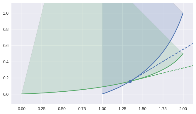
We determine the interior (i.e. left) one by using the right-hand rule: by embedding the tangent vectors in \(\mathbf{R}^3\), we compute
\[\begin{split}\left[\begin{array}{c} x_1'(s) \\ y_1'(s) \\ 0 \end{array}\right] \times \left[\begin{array}{c} x_2'(t) \\ y_2'(t) \\ 0 \end{array}\right] = \left[\begin{array}{c} 0 \\ 0 \\ x_1'(s) y_2'(t) - x_2'(t) y_1'(s) \end{array}\right].\end{split}\]If the cross product quantity \(B_1'(s) \times B_2'(t) = x_1'(s) y_2'(t) - x_2'(t) y_1'(s)\) is positive, then the first curve is “outside” / “to the right”, i.e. the second curve is interior. If the cross product is negative, the first curve is interior.
When \(B_1'(s) \times B_2'(t) = 0\), the tangent vectors are parallel, i.e. the intersection is a point of tangency:
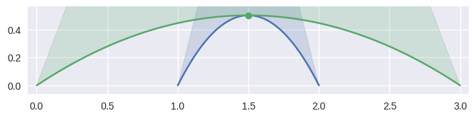
>>> nodes1 = np.asfortranarray([
...     [1.0, 0.0],
...     [1.5, 1.0],
...     [2.0, 0.0],
... ])
>>> curve1 = bezier.Curve(nodes1, degree=2)
>>> nodes2 = np.asfortranarray([
...     [0.0, 0.0],
...     [1.5, 1.0],
...     [3.0, 0.0],
... ])
>>> curve2 = bezier.Curve(nodes2, degree=2)
>>> s, t = 0.5, 0.5
>>> curve1.evaluate(s) == curve2.evaluate(t)
array([[ True, True]], dtype=bool)
>>> intersection = Intersection(curve1, s, curve2, t)
>>> classify_intersection(intersection)
<IntersectionClassification.tangent_second: 'tangent_second'>
Depending on the direction of the parameterizations, the interior curve may change, but we can use the (signed) curvature of each curve at that point to determine which is on the interior:
>>> nodes1 = np.asfortranarray([
...     [2.0, 0.0],
...     [1.5, 1.0],
...     [1.0, 0.0],
... ])
>>> curve1 = bezier.Curve(nodes1, degree=2)
>>> nodes2 = np.asfortranarray([
...     [3.0, 0.0],
...     [1.5, 1.0],
...     [0.0, 0.0],
... ])
>>> curve2 = bezier.Curve(nodes2, degree=2)
>>> s, t = 0.5, 0.5
>>> curve1.evaluate(s) == curve2.evaluate(t)
array([[ True, True]], dtype=bool)
>>> intersection = Intersection(curve1, s, curve2, t)
>>> classify_intersection(intersection)
<IntersectionClassification.tangent_first: 'tangent_first'>
When the curves are moving in opposite directions at a point of tangency, there is no side to choose. Either the point of tangency is not part of any
CurvedPolygonintersection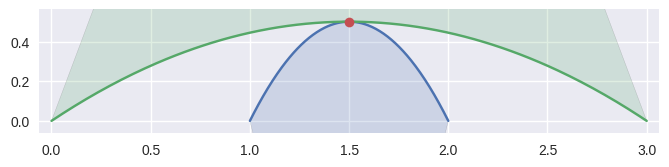
>>> nodes1 = np.asfortranarray([
...     [2.0, 0.0],
...     [1.5, 1.0],
...     [1.0, 0.0],
... ])
>>> curve1 = bezier.Curve(nodes1, degree=2)
>>> nodes2 = np.asfortranarray([
...     [0.0, 0.0],
...     [1.5, 1.0],
...     [3.0, 0.0],
... ])
>>> curve2 = bezier.Curve(nodes2, degree=2)
>>> s, t = 0.5, 0.5
>>> curve1.evaluate(s) == curve2.evaluate(t)
array([[ True, True]], dtype=bool)
>>> intersection = Intersection(curve1, s, curve2, t)
>>> classify_intersection(intersection)
<IntersectionClassification.opposed: 'opposed'>
or the point of tangency is a “degenerate” part of two
CurvedPolygonintersections. It is “degenerate” because from one direction, the point should be classified as1and from another as0: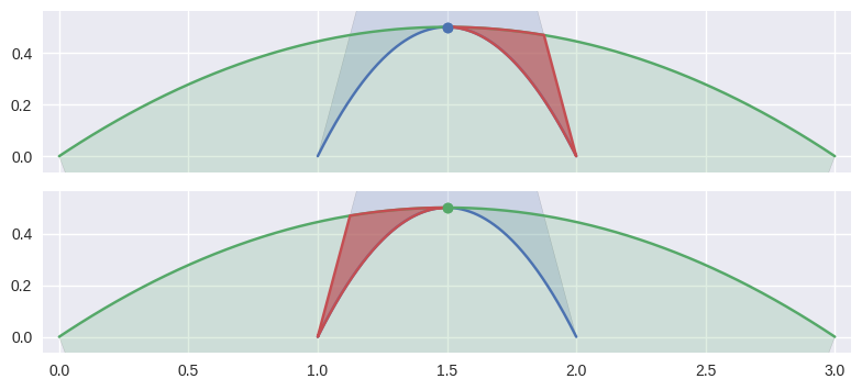
>>> nodes1 = np.asfortranarray([
...     [1.0, 0.0],
...     [1.5, 1.0],
...     [2.0, 0.0],
... ])
>>> curve1 = bezier.Curve(nodes1, degree=2)
>>> nodes2 = np.asfortranarray([
...     [3.0, 0.0],
...     [1.5, 1.0],
...     [0.0, 0.0],
... ])
>>> curve2 = bezier.Curve(nodes2, degree=2)
>>> s, t = 0.5, 0.5
>>> curve1.evaluate(s) == curve2.evaluate(t)
array([[ True, True]], dtype=bool)
>>> intersection = Intersection(curve1, s, curve2, t)
>>> classify_intersection(intersection)
Traceback (most recent call last):
  ...
NotImplementedError: Curves moving in opposite direction
                     but define overlapping arcs.
However, if the curvature of each curve is identical, we don’t try to distinguish further:
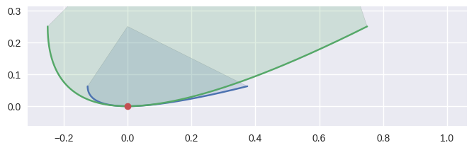
>>> nodes1 = np.asfortranarray([
...     [ 0.375,  0.0625],
...     [-0.125, -0.0625],
...     [-0.125,  0.0625],
... ])
>>> curve1 = bezier.Curve(nodes1, degree=2)
>>> nodes2 = np.asfortranarray([
...     [ 0.75,  0.25],
...     [-0.25, -0.25],
...     [-0.25,  0.25],
... ])
>>> curve2 = bezier.Curve(nodes2, degree=2)
>>> s, t = 0.5, 0.5
>>> curve1.evaluate(s) == curve2.evaluate(t)
array([[ True, True]], dtype=bool)
>>> hodograph(curve1, s)
array([[-0.5, 0. ]])
>>> hodograph(curve2, t)
array([[-1., 0.]])
>>> curvature(curve1, s)
-2.0
>>> curvature(curve2, t)
-2.0
>>> intersection = Intersection(curve1, s, curve2, t)
>>> classify_intersection(intersection)
Traceback (most recent call last):
  ...
NotImplementedError: Tangent curves have same curvature.
In addition to points of tangency, intersections that happen at the end of an edge need special handling:
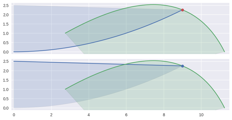
>>> nodes1a = np.asfortranarray([
...     [0.0, 0.0 ],
...     [4.5, 0.0 ],
...     [9.0, 2.25],
... ])
>>> curve1a = bezier.Curve(nodes1a, degree=2)
>>> nodes2 = np.asfortranarray([
...     [11.25, 0.0],
...     [ 9.0 , 4.5],
...     [ 2.75, 1.0],
... ])
>>> curve2 = bezier.Curve(nodes2, degree=2)
>>> s, t = 1.0, 0.375
>>> curve1a.evaluate(s) == curve2.evaluate(t)
array([[ True, True]], dtype=bool)
>>> intersection = Intersection(curve1a, s, curve2, t)
>>> classify_intersection(intersection)
Traceback (most recent call last):
  ...
ValueError: ('Intersection occurs at the end of an edge',
             's', 1.0, 't', 0.375)
>>>
>>> nodes1b = np.asfortranarray([
...     [9.0, 2.25 ],
...     [4.5, 2.375],
...     [0.0, 2.5  ],
... ])
>>> curve1b = bezier.Curve(nodes1b, degree=2)
>>> curve1b.evaluate(0.0) == curve2.evaluate(t)
array([[ True, True]], dtype=bool)
>>> curve1b._previous_edge = curve1a
>>> intersection = Intersection(curve1b, 0.0, curve2, t)
>>> classify_intersection(intersection)
<IntersectionClassification.first: 'first'>
As above, some intersections at the end of an edge are part of an actual intersection. However, some surfaces may just “kiss” at a corner intersection:
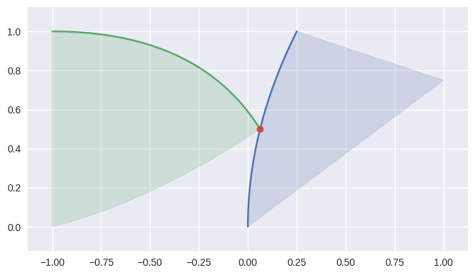
>>> nodes1 = np.asfortranarray([
...     [0.25 , 1.0  ],
...     [0.0  , 0.5  ],
...     [0.0  , 0.0  ],
...     [0.625, 0.875],
...     [0.5  , 0.375],
...     [1.0  , 0.75 ],
... ])
>>> surface1 = bezier.Surface(nodes1, degree=2)
>>> nodes2 = np.asfortranarray([
...     [ 0.0625, 0.5  ],
...     [-0.25  , 1.0  ],
...     [-1.0   , 1.0  ],
...     [-0.5   , 0.125],
...     [-1.0   , 0.5  ],
...     [-1.0   , 0.0  ],
... ])
>>> surface2 = bezier.Surface(nodes2, degree=2)
>>> curve1, _, _ = surface1.edges
>>> curve2, _, _ = surface2.edges
>>> s, t = 0.5, 0.0
>>> curve1.evaluate(s) == curve2.evaluate(t)
array([[ True, True]], dtype=bool)
>>> intersection = Intersection(curve1, s, curve2, t)
>>> classify_intersection(intersection)
<IntersectionClassification.ignored_corner: 'ignored_corner'>
Note
This assumes the intersection occurs in \(\mathbf{R}^2\) but doesn’t check this.
Note
This function doesn’t allow wiggle room / round-off when checking endpoints, nor when checking if the cross product is near zero, nor when curvatures are compared. However, the most “correct” version of this function likely should allow for some round off.
Parameters: intersection (Intersection) – An intersection object. Returns: The “inside” curve type, based on the classification enum. Return type: IntersectionClassification Raises: ValueError– If the intersection occurs at the end of either curve involved. This is because we want to classify which curve to move forward on, and we can’t move past the end of a segment.
-
bezier._surface_helpers._jacobian_det(nodes, degree, st_vals)¶ Compute \(\det(D B)\) at a set of values.
This requires that \(B \in \mathbf{R}^2\).
Note
This assumes but does not check that each
(s, t)inst_valsis inside the reference triangle.Warning
This relies on helpers in
bezierfor computing the Jacobian of the surface. However, these helpers are not part of the public surface and may change or be removed.>>> nodes = np.asfortranarray([ ... [0.0, 0.0], ... [1.0, 0.0], ... [2.0, 0.0], ... [0.0, 1.0], ... [1.5, 1.5], ... [0.0, 2.0], ... ]) >>> surface = bezier.Surface(nodes, degree=2) >>> st_vals = np.asfortranarray([ ... [0.25, 0.0 ], ... [0.75, 0.125], ... [0.5 , 0.5 ], ... ]) >>> s_vals, t_vals = st_vals.T >>> surface.evaluate_cartesian_multi(st_vals) array([[ 0.5 , 0. ], [ 1.59375, 0.34375], [ 1.25 , 1.25 ]]) >>> # B(s, t) = [s(t + 2), t(s + 2)] >>> s_vals * (t_vals + 2) array([ 0.5 , 1.59375, 1.25 ]) >>> t_vals * (s_vals + 2) array([ 0. , 0.34375, 1.25 ]) >>> jacobian_det(nodes, 2, st_vals) array([ 4.5 , 5.75, 6. ]) >>> # det(DB) = 2(s + t + 2) >>> 2 * (s_vals + t_vals + 2) array([ 4.5 , 5.75, 6. ])
Parameters: - nodes (numpy.ndarray) – Nodes defining a Bézier surface \(B(s, t)\).
- degree (int) – The degree of the surface \(B\).
- st_vals (numpy.ndarray) –
Nx2array of Cartesian inputs to Bézier surfaces defined by \(B_s\) and \(B_t\).
Returns: Array of all determinant values, one for each row in
st_vals.Return type:
-
bezier._surface_helpers._2x2_det(mat)¶ Compute the determinant of a 2x2 matrix.
This is “needed” because
numpy.linalg.det()uses a more generic determinant implementation which can introduce rounding even when the simple \(a d - b c\) will suffice. For example:>>> import numpy as np >>> mat = np.asfortranarray([ ... [-1.5 , 0.1875], ... [-1.6875, 0.0 ], ... ]) >>> actual_det = -mat[0, 1] * mat[1, 0] >>> np_det = np.linalg.det(mat) >>> np.abs(actual_det - np_det) == np.spacing(actual_det) True
Parameters: mat (numpy.ndarray) – A 2x2 matrix. Returns: The determinant of mat.Return type: float
-
bezier._implicitization.bezier_roots(coeffs)¶ Compute polynomial roots from a polynomial in the Bernstein basis.
Note
This assumes the caller passes in a 1D array but does not check.
This takes the polynomial
\[f(s) = \sum_{j = 0}^n b_{j, n} \cdot C_j.\]and uses the variable \(\sigma = \frac{s}{1 - s}\) to rewrite as
\[\begin{split}\begin{align*} f(s) &= (1 - s)^n \sum_{j = 0}^n \binom{n}{j} C_j \sigma^j \\ &= (1 - s)^n \sum_{j = 0}^n \widetilde{C_j} \sigma^j. \end{align*}\end{split}\]Then it uses an eigenvalue solver to find the roots of
\[g(\sigma) = \sum_{j = 0}^n \widetilde{C_j} \sigma^j\]and convert them back into roots of \(f(s)\) via \(s = \frac{\sigma}{1 + \sigma}\).
For example, consider
\[\begin{split}\begin{align*} f_0(s) &= 2 (2 - s)(3 + s) \\ &= 12(1 - s)^2 + 11 \cdot 2s(1 - s) + 8 s^2 \end{align*}\end{split}\]First, we compute the companion matrix for
\[g_0(\sigma) = 12 + 22 \sigma + 8 \sigma^2\]>>> coeffs0 = np.asfortranarray([12.0, 11.0, 8.0]) >>> companion0, _, _ = bernstein_companion(coeffs0) >>> companion0 array([[-2.75, -1.5 ], [ 1. , 0. ]])
then take the eigenvalues of the companion matrix:
>>> sigma_values0 = np.linalg.eigvals(companion0)
>>> sigma_values0
array([-2.  , -0.75])
after transforming them, we have the roots of \(f(s)\):
>>> sigma_values0 / (1.0 + sigma_values0)
array([ 2., -3.])
>>> bezier_roots(coeffs0)
array([ 2., -3.])
In cases where \(s = 1\) is a root, the lead coefficient of \(g\) would be \(0\), so there is a reduction in the companion matrix.
\[\begin{split}\begin{align*} f_1(s) &= 6 (s - 1)^2 (s - 3) (s - 5) \\ &= 90 (1 - s)^4 + 33 \cdot 4s(1 - s)^3 + 8 \cdot 6s^2(1 - s)^2 \end{align*}\end{split}\]>>> coeffs1 = np.asfortranarray([90.0, 33.0, 8.0, 0.0, 0.0]) >>> companion1, degree1, effective_degree1 = bernstein_companion( ... coeffs1) >>> companion1 array([[-2.75 , -1.875], [ 1. , 0. ]]) >>> degree1 4 >>> effective_degree1 2
so the roots are a combination of the roots determined from \(s = \frac{\sigma}{1 + \sigma}\) and the number of factors of \((1 - s)\) (i.e. the difference between the degree and the effective degree):
>>> bezier_roots(coeffs1)
array([ 3.,  5.,  1.,  1.])
In some cases, a polynomial is represented with an “elevated” degree:
\[\begin{split}\begin{align*} f_2(s) &= 3 (s^2 + 1) \\ &= 3 (1 - s)^3 + 3 \cdot 3s(1 - s)^2 + 4 \cdot 3s^2(1 - s) + 6 s^3 \end{align*}\end{split}\]This results in a “point at infinity” \(\sigma = -1 \Longleftrightarrow s = \infty\):
>>> coeffs2 = np.asfortranarray([3.0, 3.0, 4.0, 6.0])
>>> companion2, _, _ = bernstein_companion(coeffs2)
>>> companion2
array([[-2. , -1.5, -0.5],
       [ 1. ,  0. ,  0. ],
       [ 0. ,  1. ,  0. ]])
>>> sigma_values2 = np.linalg.eigvals(companion2)
>>> sigma_values2
array([-1.0+0.j , -0.5+0.5j, -0.5-0.5j])
so we drop any values \(\sigma\) that are sufficiently close to \(-1\):
>>> expected2 = np.asfortranarray([1.0j, -1.0j])
>>> roots2 = bezier_roots(coeffs2)
>>> np.allclose(expected2, roots2, rtol=2e-15, atol=0.0)
True
Parameters: coeffs (numpy.ndarray) – A 1D array of coefficients in the Bernstein basis. Returns: A 1D array containing the roots. Return type: numpy.ndarray
-
bezier._implicitization.lu_companion(top_row, value)¶ Compute an LU-factored \(C - t I\) and its 1-norm.
Note
The output of this function is intended to be used with
dgeconfrom LAPACK.dgeconexpects both the 1-norm of the matrix and expects the matrix to be passed in an already LU-factored form (viadgetrf).The companion matrix \(C\) is given by the
top_row, for example, the polynomial \(t^3 + 3 t^2 - t + 2\) has a top row of-3, 1, -2and the corresponding companion matrix is:\[\begin{split}\left[\begin{array}{c c c} -3 & 1 & -2 \\ 1 & 0 & 0 \\ 0 & 1 & 0 \end{array}\right]\end{split}\]After doing a full cycle of the rows (shifting the first to the last and moving all other rows up), row reduction of \(C - t I\) yields
\[\begin{split}\left[\begin{array}{c c c} 1 & -t & 0 \\ 0 & 1 & -t \\ -3 - t & 1 & -2 \end{array}\right] = \left[\begin{array}{c c c} 1 & 0 & 0 \\ 0 & 1 & 0 \\ -3 - t & 1 + t(-3 - t) & 1 \end{array}\right] \left[\begin{array}{c c c} 1 & -t & 0 \\ 0 & 1 & -t \\ 0 & 0 & -2 + t(1 + t(-3 - t)) \end{array}\right]\end{split}\]and in general, the terms in the bottom row correspond to the intermediate values involved in evaluating the polynomial via Horner’s method.
>>> top_row = np.asfortranarray([-3.0, 1.0, -2.0])
>>> t_val = 0.5
>>> lu_mat, one_norm = lu_companion(top_row, t_val)
>>> lu_mat
array([[ 1.   , -0.5  ,  0.   ],
       [ 0.   ,  1.   , -0.5  ],
       [-3.5  , -0.75 , -2.375]])
>>> one_norm
4.5
>>> l_mat = np.tril(lu_mat, k=-1) + np.eye(3)
>>> u_mat = np.triu(lu_mat)
>>> a_mat = l_mat.dot(u_mat)
>>> a_mat
array([[ 1. , -0.5,  0. ],
       [ 0. ,  1. , -0.5],
       [-3.5,  1. , -2. ]])
>>> np.linalg.norm(a_mat, ord=1)
4.5
Parameters: - top_row (numpy.ndarray) – 1D array, top row of companion matrix.
- value (float) – The \(t\) value used to form \(C - t I\).
Returns: Pair of
- 2D array of LU-factored form of \(C - t I\), with the non-diagonal part of \(L\) stored in the strictly lower triangle and \(U\) stored in the upper triangle (we skip the permutation matrix, as it won’t impact the 1-norm)
- the 1-norm the matrix \(C - t I\)
As mentioned above, these two values are meant to be used with
dgecon.Return type: Tuple[numpy.ndarray,float]
-
bezier._implicitization.bezier_value_check(coeffs, s_val, rhs_val=0.0)¶ Check if a polynomial in the Bernstein basis evaluates to a value.
This is intended to be used for root checking, i.e. for a polynomial \(f(s)\) and a particular value \(s_{\ast}\):
Is it true that \(f\left(s_{\ast}\right) = 0\)?Does so by re-stating as a matrix rank problem. As in
bezier_roots(), we can rewrite\[f(s) = (1 - s)^n g\left(\sigma\right)\]for \(\sigma = \frac{s}{1 - s}\) and \(g\left(\sigma\right)\) written in the power / monomial basis. Now, checking if \(g\left(\sigma\right) = 0\) is a matter of checking that \(\det\left(C_g - \sigma I\right) = 0\) (where \(C_g\) is the companion matrix of \(g\)).
Due to issues of numerical stability, we’d rather ask if \(C_g - \sigma I\) is singular to numerical precision. A typical approach to this using the singular values (assuming \(C_g\) is \(m \times m\)) is that the matrix is singular if
\[\sigma_m < m \varepsilon \sigma_1 \Longleftrightarrow \frac{1}{\kappa_2} < m \varepsilon\](where \(\kappa_2\) is the 2-norm condition number of the matrix). Since we also know that \(\kappa_2 < \kappa_1\), a stronger requirement would be
\[\frac{1}{\kappa_1} < \frac{1}{\kappa_2} < m \varepsilon.\]This is more useful since it is much easier to compute the 1-norm condition number / reciprocal condition number (and methods in LAPACK are provided for doing so).
Parameters: - coeffs (numpy.ndarray) – A 1D array of coefficients in the Bernstein basis representing a polynomial.
- s_val (float) – The value to check on the polynomial: \(f(s) = r\).
- rhs_val (
Optional[float]) – The value to check that the polynomial evaluates to. Defaults to0.0.
Returns: Indicates if \(f\left(s_{\ast}\right) = r\) (where \(s_{\ast}\) is
s_valand \(r\) isrhs_val).Return type: