bezier.curve module
Helper for Bézier Curves.
See Curve-Curve Intersection for examples using the
Curve class to find intersections.
-
class
bezier.curve.IntersectionStrategy¶ Enum determining if the type of intersection algorithm to use.
-
class
bezier.curve.Curve(nodes, degree, start=0.0, end=1.0, root=None, _copy=True)¶ Bases:
bezier._base.BaseRepresents a Bézier curve.
We take the traditional definition: a Bézier curve is a mapping from \(s \in \left[0, 1\right]\) to convex combinations of points \(v_0, v_1, \ldots, v_n\) in some vector space:
\[B(s) = \sum_{j = 0}^n \binom{n}{j} s^j (1 - s)^{n - j} \cdot v_j\]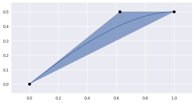
>>> import bezier
>>> nodes = np.asfortranarray([
...     [0.0  , 0.0],
...     [0.625, 0.5],
...     [1.0  , 0.5],
... ])
>>> curve = bezier.Curve.from_nodes(nodes)
>>> curve
<Curve (degree=2, dimension=2)>
Parameters: - nodes (numpy.ndarray) – The nodes in the curve. The rows represent each node while the columns are the dimension of the ambient space.
- degree (int) – The degree of the curve. This is assumed to
correctly correspond to the number of
nodes. Usefrom_nodes()if the degree has not yet been computed. - start (
Optional[float]) – The beginning of the sub-interval that this curve represents. - end (
Optional[float]) – The end of the sub-interval that this curve represents. - root (
Optional[Curve]) – The root curve that contains this current curve. - _copy (bool) – Flag indicating if the nodes should be copied before
being stored. Defaults to
Truesince callers may freely mutatenodesafter passing in.
-
degree¶ int – The degree of the current shape.
-
dimension¶ int – The dimension that the shape lives in.
For example, if the shape lives in \(\mathbf{R}^3\), then the dimension is
3.
-
edge_index¶ Optional[int] – The index of the edge among a group of edges.>>> curve.edge_index 1 >>> curve.previous_edge <Curve (degree=1, dimension=2)> >>> curve.previous_edge.edge_index 0 >>> curve.next_edge <Curve (degree=1, dimension=2)> >>> curve.next_edge.edge_index 2
This is intended to be used when a
Curveis created as part of a larger structure like aSurfaceorCurvedPolygon.
-
elevate()¶ Return a degree-elevated version of the current curve.
Does this by converting the current nodes \(v_0, \ldots, v_n\) to new nodes \(w_0, \ldots, w_{n + 1}\) where
\[\begin{split}\begin{align*} w_0 &= v_0 \\ w_j &= \frac{j}{n + 1} v_{j - 1} + \frac{n + 1 - j}{n + 1} v_j \\ w_{n + 1} &= v_n \end{align*}\end{split}\]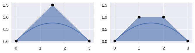
>>> nodes = np.asfortranarray([
...     [0.0, 0.0],
...     [1.5, 1.5],
...     [3.0, 0.0],
... ])
>>> curve = bezier.Curve(nodes, degree=2)
>>> elevated = curve.elevate()
>>> elevated
<Curve (degree=3, dimension=2)>
>>> elevated.nodes
array([[ 0., 0.],
       [ 1., 1.],
       [ 2., 1.],
       [ 3., 0.]])
Returns: The degree-elevated curve. Return type: Curve
-
evaluate(s)¶ Evaluate \(B(s)\) along the curve.
See
evaluate_multi()for more details.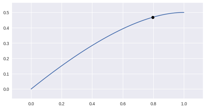
>>> nodes = np.asfortranarray([
...     [0.0  , 0.0],
...     [0.625, 0.5],
...     [1.0  , 0.5],
... ])
>>> curve = bezier.Curve(nodes, degree=2)
>>> curve.evaluate(0.75)
array([[ 0.796875, 0.46875 ]])
Parameters: s (float) – Parameter along the curve. Returns: The point on the curve (as a two dimensional NumPy array with a single row). Return type: numpy.ndarray
-
evaluate_multi(s_vals)¶ Evaluate \(B(s)\) for multiple points along the curve.
This is done via a modified Horner’s method (vectorized for each
s-value).>>> nodes = np.asfortranarray([ ... [0.0, 0.0, 0.0], ... [1.0, 2.0, 3.0], ... ]) >>> curve = bezier.Curve(nodes, degree=1) >>> curve <Curve (degree=1, dimension=3)> >>> s_vals = np.linspace(0.0, 1.0, 5) >>> curve.evaluate_multi(s_vals) array([[ 0. , 0. , 0. ], [ 0.25, 0.5 , 0.75], [ 0.5 , 1. , 1.5 ], [ 0.75, 1.5 , 2.25], [ 1. , 2. , 3. ]])
Parameters: s_vals (numpy.ndarray) – Parameters along the curve (as a 1D array). Returns: The points on the curve. As a two dimensional NumPy array, with the rows corresponding to each svalue and the columns to the dimension.Return type: numpy.ndarray
-
classmethod
from_nodes(nodes, start=0.0, end=1.0, root=None, _copy=True)¶ Create a
Curvefrom nodes.Computes the
degreebased on the shape ofnodes.Parameters: - nodes (numpy.ndarray) – The nodes in the curve. The rows represent each node while the columns are the dimension of the ambient space.
- start (
Optional[float]) – The beginning of the sub-interval that this curve represents. - end (
Optional[float]) – The end of the sub-interval that this curve represents. - root (
Optional[Curve]) – The root curve that contains this current curve. - _copy (bool) – Flag indicating if the nodes should be copied before
being stored. Defaults to
Truesince callers may freely mutatenodesafter passing in.
Returns: The constructed curve.
Return type:
-
intersect(other, strategy=<IntersectionStrategy.geometric: 'geometric'>, _verify=True)¶ Find the points of intersection with another curve.
See Curve-Curve Intersection for more details.
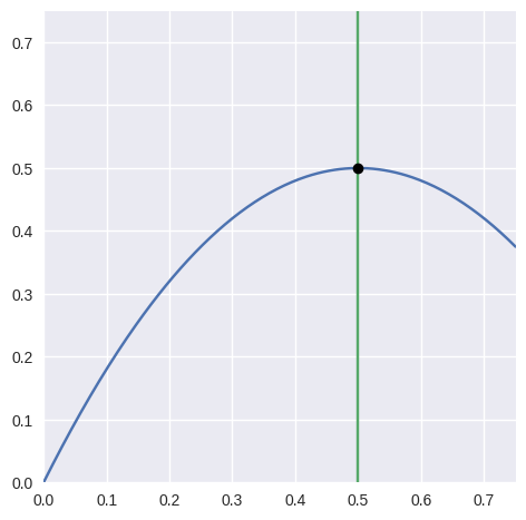
>>> nodes1 = np.asfortranarray([
...     [0.0  , 0.0  ],
...     [0.375, 0.75 ],
...     [0.75 , 0.375],
... ])
>>> curve1 = bezier.Curve(nodes1, degree=2)
>>> nodes2 = np.asfortranarray([
...     [0.5, 0.0 ],
...     [0.5, 0.75],
... ])
>>> curve2 = bezier.Curve(nodes2, degree=1)
>>> intersections = curve1.intersect(curve2)
>>> intersections
array([[ 0.5, 0.5]])
Parameters: - other (Curve) – Other curve to intersect with.
- strategy (
Optional[IntersectionStrategy]) – The intersection algorithm to use. Defaults to geometric. - _verify (
Optional[bool]) – Indicates if extra caution should be used to verify assumptions about the input and current curve. Can be disabled to speed up execution time. Defaults toTrue.
Returns: Array of intersection points (possibly empty).
Return type: Raises: TypeError– Ifotheris not a curve (and_verify=True).NotImplementedError– If at least one of the curves isn’t two-dimensional (and_verify=True).
-
length¶ float – The length of the current curve.
-
locate(point)¶ Find a point on the current curve.
Solves for \(s\) in \(B(s) = p\).
Note
A unique solution is only guaranteed if the current curve has no self-intersections. This code assumes, but doesn’t check, that this is true.
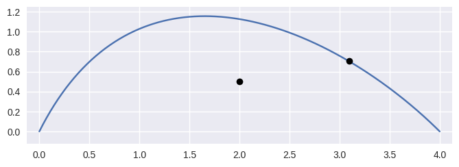
>>> nodes = np.asfortranarray([
...     [0.0, 0.0],
...     [1.0, 2.0],
...     [3.0, 1.0],
...     [4.0, 0.0],
... ])
>>> curve = bezier.Curve(nodes, degree=3)
>>> point1 = np.asfortranarray([[3.09375, 0.703125]])
>>> s = curve.locate(point1)
>>> s
0.75
>>> point2 = np.asfortranarray([[2.0, 0.5]])
>>> curve.locate(point2) is None
True
Parameters: point (numpy.ndarray) – A ( 1xD) point on the curve, where \(D\) is the dimension of the curve.Returns: The parameter value (\(s\)) corresponding to pointorNoneif the point is not on thecurve.Return type: Optional[float]Raises: ValueError– If the dimension of thepointdoesn’t match the dimension of the current curve.
-
next_edge¶ Optional[Curve] – An edge that comes after the current one.This is intended to be used when a
Curveis created as part of a larger structure like aSurfaceorCurvedPolygon.
-
nodes¶ numpy.ndarray – The nodes that define the current shape.
-
plot(num_pts, color=None, alpha=None, ax=None)¶ Plot the current curve.
Parameters: Returns: The axis containing the plot. This may be a newly created axis.
Return type: Raises: NotImplementedError– If the curve’s dimension is not2.
-
previous_edge¶ Optional[Curve] – An edge that comes before the current one.This is intended to be used when a
Curveis created as part of a larger structure like aSurfaceorCurvedPolygon.
-
reduce_()¶ Return a degree-reduced version of the current curve.
Does this by converting the current nodes \(v_0, \ldots, v_n\) to new nodes \(w_0, \ldots, w_{n - 1}\) that correspond to reversing the
elevate()process.This uses the pseudo-inverse of the elevation matrix. For example when elevating from degree 2 to 3, the matrix \(E_2\) is given by
\[\begin{split}\mathbf{v} = \left[\begin{array}{c} v_0 \\ v_1 \\ v_2 \end{array}\right] \longmapsto \left[\begin{array}{c} v_0 \\ \frac{v_0 + 2 v_1}{3} \\ \frac{2 v_1 + v_2}{3} \\ v_2 \end{array}\right] = \frac{1}{3} \left[\begin{array}{c c} 3 & 0 \\ 2 & 1 \\ 1 & 2 \\ 0 & 3 \end{array}\right] \mathbf{v}\end{split}\]and the pseudo-inverse is given by
\[\begin{split}R_2 = \left(E_2^T E_2\right)^{-1} E_2^T = \frac{1}{20} \left[\begin{array}{c c c c} 19 & 3 & -3 & 1 \\ -5 & 15 & 15 & -5 \\ 1 & -3 & 3 & 19 \end{array}\right].\end{split}\]Warning
Though degree-elevation preserves the start and end nodes, degree reduction has no such guarantee. Rather, the nodes produced are “best” in the least squares sense (when solving the normal equations).
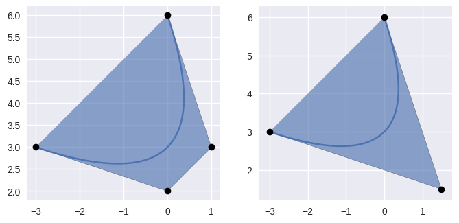
>>> nodes = np.asfortranarray([
...     [-3.0, 3.0],
...     [ 0.0, 2.0],
...     [ 1.0, 3.0],
...     [ 0.0, 6.0],
... ])
>>> curve = bezier.Curve(nodes, degree=3)
>>> reduced = curve.reduce_()
>>> reduced
<Curve (degree=2, dimension=2)>
>>> reduced.nodes
array([[-3. , 3. ],
       [ 1.5, 1.5],
       [ 0. , 6. ]])
In the case that the current curve is not degree-elevated.
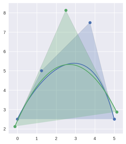
>>> nodes = np.asfortranarray([
...     [0.0 , 2.5],
...     [1.25, 5.0],
...     [3.75, 7.5],
...     [5.0 , 2.5],
... ])
>>> curve = bezier.Curve(nodes, degree=3)
>>> reduced = curve.reduce_()
>>> reduced
<Curve (degree=2, dimension=2)>
>>> reduced.nodes
array([[-0.125, 2.125],
       [ 2.5  , 8.125],
       [ 5.125, 2.875]])
Returns: The degree-reduced curve. Return type: Curve
-
root¶ Curve – The “root” curve that contains the current curve.
This indicates that the current curve is a section of the “root” curve. For example:
>>> _, right = curve.subdivide()
>>> right
<Curve (degree=2, dimension=2, start=0.5, end=1)>
>>> right.root is curve
True
>>> right.evaluate(0.0) == curve.evaluate(0.5)
array([[ True, True]], dtype=bool)
>>>
>>> mid_left, _ = right.subdivide()
>>> mid_left
<Curve (degree=2, dimension=2, start=0.5, end=0.75)>
>>> mid_left.root is curve
True
>>> mid_left.evaluate(1.0) == curve.evaluate(0.75)
array([[ True, True]], dtype=bool)
-
specialize(start, end)¶ Specialize the curve to a given sub-interval.
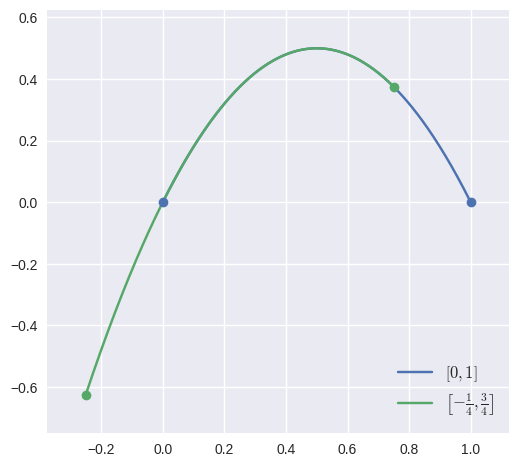
>>> nodes = np.asfortranarray([
...     [0.0, 0.0],
...     [0.5, 1.0],
...     [1.0, 0.0],
... ])
>>> curve = bezier.Curve(nodes, degree=2)
>>> new_curve = curve.specialize(-0.25, 0.75)
>>> new_curve
<Curve (degree=2, dimension=2, start=-0.25, end=0.75)>
>>> new_curve.nodes
array([[-0.25 , -0.625],
       [ 0.25 ,  0.875],
       [ 0.75 ,  0.375]])
This is generalized version of
subdivide(), and can even match the output of that method:>>> left, right = curve.subdivide() >>> also_left = curve.specialize(0.0, 0.5) >>> np.all(also_left.nodes == left.nodes) True >>> also_right = curve.specialize(0.5, 1.0) >>> np.all(also_right.nodes == right.nodes) True
Parameters: Returns: The newly-specialized curve.
Return type:
-
start¶ float – Start of sub-interval this curve represents.
This value is used to track the current curve in the re-parameterization / subdivision process. The curve is still defined on the unit interval, but this value illustrates how this curve relates to a “parent” curve. For example:
>>> nodes = np.asfortranarray([
...     [0.0, 0.0],
...     [1.0, 2.0],
... ])
>>> curve = bezier.Curve(nodes, degree=1)
>>> curve
<Curve (degree=1, dimension=2)>
>>> left, right = curve.subdivide()
>>> left
<Curve (degree=1, dimension=2, start=0, end=0.5)>
>>> right
<Curve (degree=1, dimension=2, start=0.5, end=1)>
>>> _, mid_right = left.subdivide()
>>> mid_right
<Curve (degree=1, dimension=2, start=0.25, end=0.5)>
>>> mid_right.nodes
array([[ 0.25, 0.5 ],
       [ 0.5 , 1.  ]])
-
subdivide()¶ Split the curve \(B(s)\) into a left and right half.
Takes the interval \(\left[0, 1\right]\) and splits the curve into \(B_1 = B\left(\left[0, \frac{1}{2}\right]\right)\) and \(B_2 = B\left(\left[\frac{1}{2}, 1\right]\right)\). In order to do this, also reparameterizes the curve, hence the resulting left and right halves have new nodes.
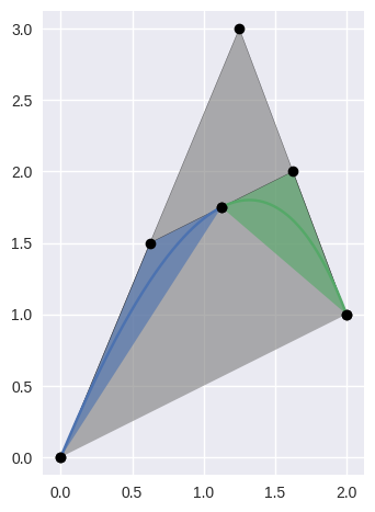
>>> nodes = np.asfortranarray([
...     [0.0 , 0.0],
...     [1.25, 3.0],
...     [2.0 , 1.0],
... ])
>>> curve = bezier.Curve(nodes, degree=2)
>>> left, right = curve.subdivide()
>>> left
<Curve (degree=2, dimension=2, start=0, end=0.5)>
>>> left.nodes
array([[ 0.   , 0.   ],
       [ 0.625, 1.5  ],
       [ 1.125, 1.75 ]])
>>> right
<Curve (degree=2, dimension=2, start=0.5, end=1)>
>>> right.nodes
array([[ 1.125, 1.75 ],
       [ 1.625, 2.   ],
       [ 2.   , 1.   ]])
Returns: The left and right sub-curves. Return type: Tuple[Curve,Curve]